Nightside clouds and disequilibrium chemistry on the hot Jupiter WASP-43b

Abstract

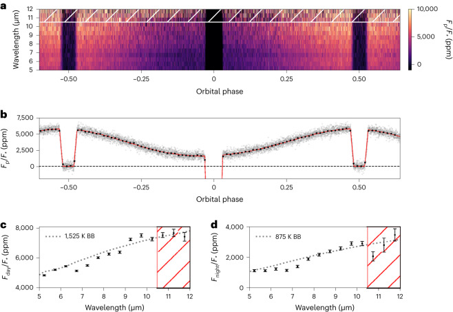
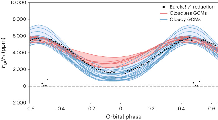
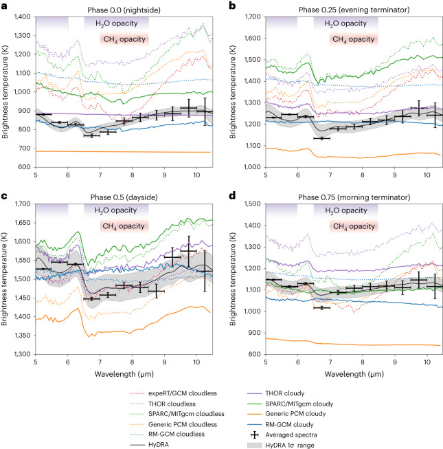
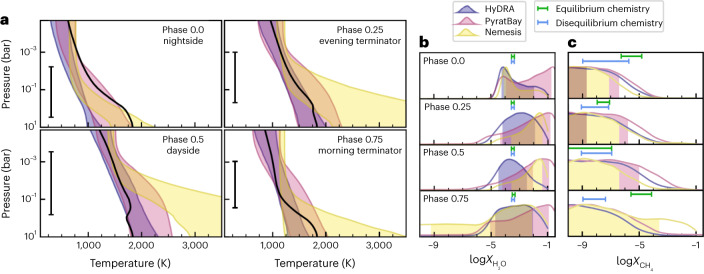
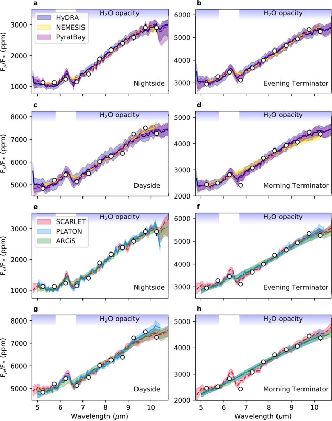
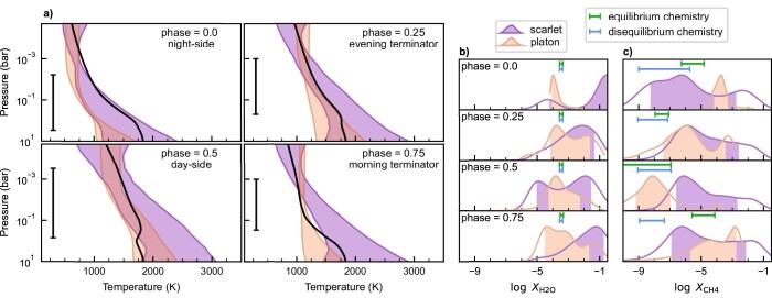
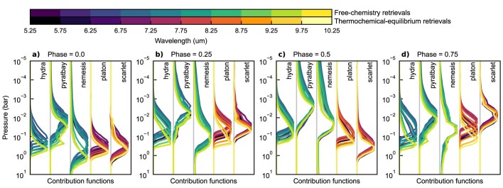
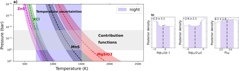
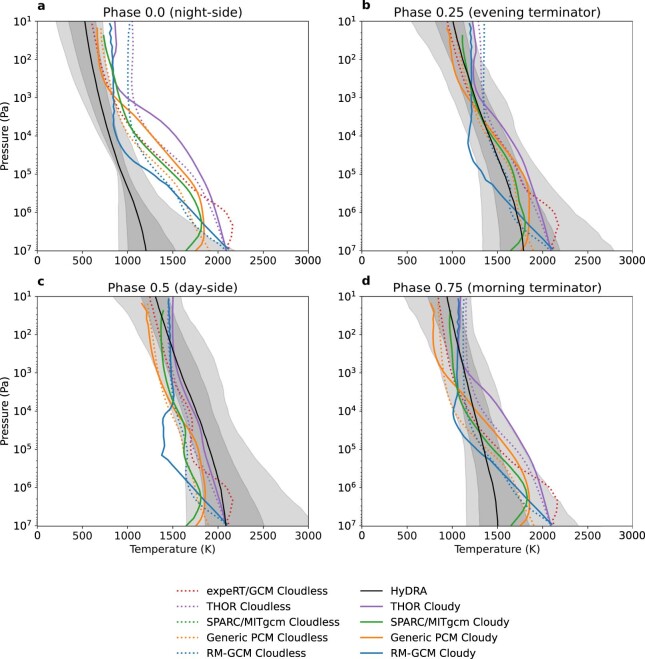
Hot Jupiters are among the best-studied exoplanets, but it is still poorly understood how their chemical composition and cloud properties vary with longitude. Theoretical models predict that clouds may condense on the nightside and that molecular abundances can be driven out of equilibrium by zonal winds. Here we report a phase-resolved emission spectrum of the hot Jupiter WASP-43b measured from 5 μm to 12 μm with the JWST's Mid-Infrared Instrument. The spectra reveal a large day-night temperature contrast (with average brightness temperatures of 1,524 ± 35 K and 863 ± 23 K, respectively) and evidence for water absorption at all orbital phases. Comparisons with three-dimensional atmospheric models show that both the phase-curve shape and emission spectra strongly suggest the presence of nightside clouds that become optically thick to thermal emission at pressures greater than ~100 mbar. The dayside is consistent with a cloudless atmosphere above the mid-infrared photosphere. Contrary to expectations from equilibrium chemistry but consistent with disequilibrium kinetics models, methane is not detected on the nightside (2σ upper limit of 1-6 ppm, depending on model assumptions). Our results provide strong evidence that the atmosphere of WASP-43b is shaped by disequilibrium processes and provide new insights into the properties of the planet's nightside clouds. However, the remaining discrepancies between our observations and our predictive atmospheric models emphasize the importance of further exploring the effects of clouds and disequilibrium chemistry in numerical models.

Keywords: Exoplanets.

Fig. 1. A visualization of the observed light curves and the resulting emission spectra.

a, The observed spectroscopic light curves binned to a 0.5 μm wavelength resolution and after systematic noise removal, following the Eureka! v1 methods. The first 779 integrations have been removed from this figure and our fits as they were impacted by strongly decreasing flux. Wavelengths longer than 10.5 μm marked with a hatched region were affected by the ‘shadowed region effect’ (Methods) and could not be reliably reduced. b, The observed band-integrated light curve after systematic noise removal (grey points) and binned data with a cadence of 15 min (black points, with error bars smaller than the point sizes), compared with the best-fitting astrophysical model (red line). c,d, The measured dayside (c) and nightside (d) emission spectra are shown with black points and 1σ error bars, and black-body curves (dotted line denoted as ‘BB’, assuming a PHOENIX^– model for the star) are shown to emphasize planetary spectral features with black-body temperatures estimated by eye to match the continuum flux levels. Wavelengths longer than 10.5 μm were affected by the shadowed region effect and are unreliable.

Fig. 2. A comparison of the observed 5–10.5 μm light curve with GCM simulations.

The black points show the temporally binned broadband light curve. The solid lines represent modelled phase curves derived from the 31 GCM simulations, integrated over the same wavelength range as the data, and separated into two groups based on the inclusion of clouds. The cloudless GCMs (red lines) simulated completely cloud-free skies, whereas the cloudy GCMs (blue lines) included at least some clouds on the nightside of the planet. The red and blue shaded areas span the range of all the cloudless and cloudy simulations, respectively, with the spread of values owing to differences in the various model assumptions and parameterizations. On average, the cloudless GCM phase curves have a maximum planet-to-star flux ratio of 5,703 ppm and a minimum of 2,681 ppm. This matches the observed maximum of the phase curve well but does not match its observed minimum at 1,636 ± 37 ppm. On average, the cloudy GCM phase curves have a maximum of 5,866 ppm and a minimum of 1,201 ppm, in better agreement with the observed nightside emission, but their spread of maximum values is much larger than the cloudless simulations. The cloudy models are able to suppress the nightside emission and better match the data; however, not all cloud models fit equally well and those with the optically thickest nightside clouds suppress too much emission. The models do not include the eclipse signals (phases −0.5 and 0.5) or transit signal (phase 0.0).

Fig. 3. A comparison of the observed and modelled spectra at different phases.

a–c, The observed emission spectrum with 1σ error bars at phases 0.0 (a), 0.25 (b), 0.5 (c) and 0.75 (d), along with select modelled spectra derived from different cloudy and cloudless GCMs (described in Methods and listed in Extended Data Table 1). Although absolute brightness temperatures differ appreciably between models owing to various GCM assumptions, differences in the relative shape of the spectra are strongly dependent on the cloud and temperature structure found in the GCMs (Extended Data Fig. 7). Models with more isothermal profiles (like RM-GCM) or thick clouds at pressures of ≲10–100 mbar (like THOR cloudy, Generic PCM with 0.1 μm cloud particles) produce flatter spectra, while clearer skies yield stronger absorption features. The observed spectra from the nightside and terminators appear muted compared with the clear-model spectra, suggesting the presence of at least some clouds or weak vertical temperature gradients at pressures of ≲10–100 mbar. In contrast, the spectral structure produced by water vapour opacity (indicated by the purple shading) appears more consistent with models lacking clouds at these low pressures on the dayside. Under equilibrium chemistry, methane would also show an absorption feature at ~7.5–8.5 μm (shaded pink) for the colder models at phases 0.0 and 0.75. Finally, the median retrieved spectrum and 1σ contours from the HyDRA retrieval are shown in grey.

Fig. 4. Atmospheric spectral retrievals for frameworks with free chemistry.

a, Temperature profile contours (68% confidence) constrained by the retrievals at each orbital phase (see legends). All frameworks produced consistent non-inverted thermal profiles that are consistent with two-dimensional radiative–convective equilibrium and photochemical models along the equator (black curves) over the range of pressures probed by the observations (black bars). b, H₂O abundance posterior distributions (volume mixing ratios). The shaded areas denote the span of the 68% confidence intervals. The green and blue bars on each panel denote the abundances predicted by equilibrium and disequilibrium chemistry solar-abundance models, respectively, at the pressures probed by the observations (1–10⁻³ bar, approximately). c, The same as in b but for CH₄. The retrieved water abundances are consistent with either equilibrium or disequilibrium chemistry estimations for solar composition (500 ppm), whereas the retrieved upper limits to the CH₄ abundance are more consistent with disequilibrium chemistry predictions.

Extended Data Fig. 1. The underestimation of uncertainties as a function of spectral binning for the L168-9b commissioning observations.

a, The observed L168-9b transmission spectrum with 1σ error bars for spectrally unbinned data (grey circles), 0.15 μm bins (black squares), 0.5 μm bins (large red circles), and a 5-12 μm broadband bin (horizontal blue shaded region). The spectrum for wavelength pairs is not shown to avoid excessive clutter. b, The median of the transit depth uncertainties are shown with blue squares, while the observed scatter in the transmission spectrum is shown with orange circles. For unbinned data, the transmission spectrum shows about 2.5 × the scatter predicted by the fits to the individual light curves. Binning pairs of wavelengths reduces the level of underestimation of the scatter in the transmission spectrum, but considerable excess noise remains. Coarser binning schemes like the constant 0.15 μm bins used in the MIRI time-series observation commissioning paper or the 0.5 μm bins we use in this work further reduce the level of uncertainty underestimation.

Extended Data Fig. 2. A model-independent demonstration of the initial changes in flux for the WASP-43b observations.

a, The first 120 minutes of three of our spectroscopically binned light curves of WASP-43b (with 1σ uncertainties) showing the initial settling behaviour as a function of wavelength. A teal dashed line shows the amplitude of a -0.25% change in flux compared to the values around 120 minutes, and a magenta dotted line shows a +0.25% change. b, A summary of the ramp amplitudes, signs, and timescales for each of our wavelength bins (with 1σ uncertainties). The teal and magenta horizontal lines are the same as those in panel a to aid in translating between the two figures. At short wavelengths, the flux sharply drops by about 0.5% within the first 30 minutes and then largely settles but does continue to decrease with time. With increasing wavelength, the strength of this initial ramp decreases and eventually changes sign, becoming an upwards ramp. Within the ‘shadowed region’ (marked in red), the light curves show a very strong upwards ramp that takes much longer (greater than about 60 minutes) to appreciably decay. It is important to note that the data in this figure also includes a small amount of astrophysical phase variations which should result in a small increase in flux of less than 0.05% per hour.

Extended Data Fig. 3. Retrieved spectra from the six retrievals.

a, Median retrieved nightside spectra for the HyDRA (dark blue line), NEMESIS (dash-dotted gold line), and PyratBay (dashed magenta line) and their 1σ contour. The regions of higher water opacity are indicated by the purple shading at the top of the panel, with the observed rise in flux at 6.3 μm being caused by a drop in opacity. b, c, and d, Same as panel a for the evening terminator, dayside, and morning terminator respectively. e, f, g, and h, Same as panels a, b, c, and d, for the SCARLET (dashed red line), PLATON (blue line), and ARCiS (dash-dotted green line) retrievals.

Extended Data Fig. 4. Chemically-consistent atmospheric retrievals.

Same as Figure 4 but for retrievals assuming thermochemical-equilibrium abundances consistent with the pressure-temperature profiles. a, 1σ credible interval contours of the temperature profiles. The black curves show the predicted temperature profile from a 2D radiative-transport model46. The vertical bars show the range of pressures probed by the observations. b and c, probability posterior distributions for H₂O and CH₄ abundances, respectively. The shaded area for each curve denotes the 1σ credible interval of each posterior. The green and blue bars denote the abundances predicted by equilibrium and disequilibrium-chemistry models with solar abundances, respectively, at the pressures probed by the observations. Compared to the free-chemistry retrievals, the thermochemical-equilibrium retrievals on the nightside spectra produced worse fits, this is driven particularly by the higher amount of methane expected under equilibrium chemistry.

Extended Data Fig. 5. Retrieval contribution functions.

Contribution functions integrated over the data point spectral bins, at each phase (a-d), and for each retrieval framework. These curves show the range of pressures probed by the observation according to the atmospheric models. The enhanced opacity from the water band around 7-9 μm makes these wavelengths probe lower pressures and hence colder temperatures, whereas the rest of the observing window probes higher pressures and higher temperatures.

Extended Data Fig. 6. PyratBay clouds exploration.

a, Cloud species that condense in the temperature regime expected for the WASP-43b nightside. Dashed lines represent vapour pressure curves for each species assuming solar composition, while the coloured ranges denote the corresponding extent of the vapour pressure curves assuming 100 × sub- and super-solar atmospheric composition. The extent of the retrieved nightside contribution functions is shown in grey, and the extent of the retrieved temperature uncertainties is shown in light purple. The intersection between the contribution function and temperature ranges indicates the pressures at which we could observe cloud condensation and potentially detect their spectral features, if present in the observations. b, Panels display the retrieved posterior density plots for the explored cloud parameters of the TSC model (cloud number density, q*; effective particle size, r_eff; and the standard deviation of the log-normal distribution, ${\sigma }_{\log }$) for the MnS clouds. The black vertical line denotes the parameter’s median value, while the extent of the purple region denotes the 1σ uncertainties, both given at the top left corner of the panel. Similar, fully non-constrained posteriors are retrieved for other explored cloud species, MgSiO₃, ZnS, and KCl, suggesting the lack of observable spectral characteristics from clouds in the observed data.

Extended Data Fig. 7. A comparison of the retrieved temperature-pressure profiles to the GCM simulations.

Each of a-d shows the temperature profile retrieved by HyDRA, compared to the GCM simulations highlighted in Figure 3 and listed in Extended Data Table 1. The GCM temperature profiles are calculated at phases 0.0, 0.25, 0.5, and 0.75 by averaging over the visible hemisphere by viewing angle, to produce a one-dimensional profile that is comparable to the retrieved profile. The GCM simulations are generally warmer on the nightside than the retrieved temperatures; cloudy simulations emit from lower pressures and so match the observed lower brightness temperatures better (see the contribution functions in Extended Data Fig. 5).

References

1. Keating, D., Cowan, N. B. & Dang, L. Uniformly hot nightside temperatures on short-period gas giants. Nat. Astron.3, 1092–1098 (2019).
1. Beatty, T. G. et al. Spitzer phase curves of KELT-1b and the signatures of nightside clouds in thermal phase observations. Astron. J.158, 166 (2019).
1. Kataria, T. et al. The atmospheric circulation of the hot Jupiter WASP-43b: comparing three-dimensional models to spectrophotometric data. Astrophys. J.801, 86 (2015).
1. Mendonça, J. M., Malik, M., Demory, B.-O. & Heng, K. Revisiting the phase curves of WASP-43b: confronting re-analyzed Spitzer data with cloudy atmospheres. Astron. J.155, 150 (2018).
1. Parmentier, V. & Crossfield, I. J. M. in Handbook of Exoplanets (eds Deeg, H. J. & Belmonte, J. A.) 1419–1440 (Springer, 2018).