Extensive structural rearrangement of intraflagellar transport trains underpins bidirectional cargo transport

Abstract

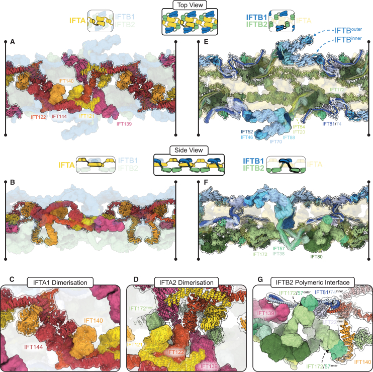
Bidirectional transport in cilia is carried out by polymers of the IFTA and IFTB protein complexes, called anterograde and retrograde intraflagellar transport (IFT) trains. Anterograde trains deliver cargoes from the cell to the cilium tip, then convert into retrograde trains for cargo export. We set out to understand how the IFT complexes can perform these two directly opposing roles before and after conversion. We use cryoelectron tomography and in situ cross-linking mass spectrometry to determine the structure of retrograde IFT trains and compare it with the known structure of anterograde trains. The retrograde train is a 2-fold symmetric polymer organized around a central thread of IFTA complexes. We conclude that anterograde-to-retrograde remodeling involves global rearrangements of the IFTA/B complexes and requires complete disassembly of the anterograde train. Finally, we describe how conformational changes to cargo-binding sites facilitate unidirectional cargo transport in a bidirectional system.

Keywords: cilia; cryoelectron tomography; intraflagellar transport; molecular structure; retrograde transport.

Graphical abstract

Figure 1

A molecular model of the retrograde IFT train (A) Slice through denoised cryoelectron tomogram of a wild-type C. reinhartii cilium, showing an anterograde IFT train sitting between the membrane (Mem) and microtubule (MT) doublet. Cartoon inset: IFTA, yellow; IFTB, blue; autoinhibited dynein-2, purple; kinesin, orange; cargo, pink. Scale bars, 25 nm. (B) Slice through denoised cryoelectron tomogram of a wild-type C. reinhartii cilium, showing a retrograde IFT train sitting between the membrane (Mem) and microtubule (MT) doublet. White arrows indicate equivalent structures in the repeat, with a spacing of ∼45 nm. Cartoon inset as in (A), but with different cargoes, brown. Scale bars, 25 nm. (C) A side view of the retrograde train density (microtubule below, membrane above), with the molecular model docked. The density becomes increasingly transparent from left to right. (D) Top view of (C), as if looking down from the membrane. Yellow stars indicate the center of rotation for the two C2 symmetry axes. See also Figure S1.

Figure S1

Cryo-ET and subtomogram averaging of wild-type and Dhc1b-3 retrograde trains, related to Figure 1 (A) Side view slice through the wild-type retrograde train average. (B) Top view of (A), as if viewing down from the membrane. (C) Fourier shell correlation (FSC) plot for the 30.3 Å wild-type average. (D) A slice through a Dhc1b-3 tomogram, indicating long rafts of repeating retrograde train structures (white arrows). Scale bar corresponds to 25 nm. (E) Fourier shell correlation (FSC) plot for the 17 Å Dhc1b-3 IFTA1 average. (F) Fourier shell correlation (FSC) plot for the 17 Å Dhc1b-3 IFTA2 average. (G) Fourier shell correlation (FSC) plot for the 18 Å Dhc1b-3 IFTB1^prox average. (H) Fourier shell correlation (FSC) plot for the 28 Å Dhc1b-3 IFTB1^dist average. (I) Fourier shell correlation (FSC) plot for the 15 Å Dhc1b-3 IFTB2 average.

Figure 2

IFTA forms the core of the retrograde train and establishes C2 symmetry (A) Top view of the retrograde train as if looking down from the membrane, highlighting the IFTA complexes. IFTA is shown in ribbon representation, with a single central complex highlighted with a semi-opaque surface. IFTB is shown as a semi-transparent surface. (B) Side view of (A), with the membrane on top and the microtubule below. (C) Close up of the IFTA1 dimerization interface. Two copies of IFT144/140 are shown, with adjacent IFTA complexes depicted with different surface opacity. (D) Close up of the IFTA2 dimerization interface. Two copies of IFT144/140/139 are shown, with adjacent IFTA complexes depicted with different surface opacity. IFT172^inner is also present. (E) Top view of the retrograde IFT model as if looking down from the membrane, highlighting IFTB complexes at the periphery of the train. IFTB complexes are shown in ribbon representation, with one pair of IFTB complexes from one repeating unit also depicted with a semi-opaque surface. IFTA complexes are shown as a transparent surface. (F) Side view of (E), with the membrane on top and microtubule below. (G) Close up of the IFTB2 polymeric interface, with one repeating unit shown with semi-opaque surfaces and the other transparent. The two copies of IFT172/57 from IFTB2 adopt different conformations to form two separate interactions with the adjacent repeat. See also Figure S2.

Figure 3

IFTA and IFTB are rearranged in retrograde trains (A) Top view of the anterograde train, with a microtubule doublet beneath in gray. (B) Top view of the retrograde train, with a microtubule doublet beneath in gray. The same number of IFTA/B complexes are shown as in the anterograde train in (A), but the length of the train is ∼70% longer. (C) Side view of the anterograde train, with the microtubule below and the membrane above. One IFTA complex and two IFTB complexes (equivalent to a repeating unit in the retrograde train) are highlighted. (D) Side view of the retrograde train, with one repeating unit highlighted. Compared with (C), the IFT complexes have undergone large movements relative to the microtubule and each other. (E) Cross-section view of the anterograde train, as if looking down the microtubule. IFTA sits on top of a platform of IFTB. (F) One repeating unit of the retrograde train, aligned so that the IFTA complex is oriented the same as in (E). The IFTB complexes have rotated 180° relative to the IFTA and are now wrapped around the IFTA. See also Figure S2.

Figure S2

Structural analyses of the retrograde train, related to Figures 2, 3, and 4 (A) Top view of the retrograde train as if looking down from the membrane. One repeating unit is shown with an opaque surface. The IFTA complex is colored yellow. IFTB^inner and IFTB^outer are differentiated by different shades of blue. (B) Side view of (A), as if the membrane is above and the microtubule is below. (C) One central repeating unit (black, corresponding to one IFTA complex and the two IFTB complexes attached to it) makes contact with four surrounding repeating units (colored with different shades of gray). Only repeating unit 4 does not interact with the central repeating unit 0. (D) Close-up views of each other interactions between IFTA and IFTB in one repeating unit of the retrograde train, shown docked into the experimental density. (E) Comparison between IFTA1 (IFT144, red, IFT140, orange) in the anterograde (transparent) and retrograde (opaque) conformations. The two models are aligned to the IFT144 WD domain. Movement of the IFT144 TPR domain associated with bridge formation has moved the IFT140 WD domains closer to the IFT144 WD domains.

Figure 4

Internal stabilization of IFTA by the bridge is required for retrograde polymerization (A) A side view of a single IFTA complex from the anterograde train. Here, IFT144 (red) and IFT121 (yellow) are distant. (B) A single IFTA complex from the retrograde train, showing the formation of the bridge. The IFT144 (red) C terminus has now moved up to contact the IFT121 (yellow) TPR region, thus stabilizing the IFTA1 and IFTA2 lobes relative to each other. (C) A top view of a single IFTA complex from the retrograde train (opaque) superimposed with the anterograde train (transparent), showing the other changes in the two structures beyond the formation of the bridge. IFTA1 (IFT144/140, red/orange) swings around to be planar with IFTA2 (IFT121/122/139, yellow/dark orange/pink), and IFT139 (pink) straightens relative to the rest of the complex. (D) Comparison between the retrograde IFTA model (opaque) and PDB: 8FGW, a cryo-EM structure of purified human IFTA (transparent). Inset, the bridge is formed in this structure, with its formation resulting in IFTA1 and IFT139 adopting the same conformations as in the retrograde train. (E) Comparison between the retrograde IFTA model (opaque) and PDB: 8F5O, a cryo-EM structure of purified Leishmania IFTA (transparent). Inset, the bridge is not formed in this structure, resulting in a kinked IFT139 conformation and IFTA1 and IFTA2 not being in a retrograde conformation. (F) Left: the IFTA1 dimerization interface experimental density with the anterograde IFTA model docked in. The open conformation of IFTA1 prevents the dimerization of IFTA1, thus preventing polymerization. Right: the same view with the refined retrograde model docked in, showing the tight dimerization interface. (G) Left: close up of the interaction between IFT139 and IFTB. The experimental density is shown with the refined retrograde IFTB model docked in. The anterograde IFTA model shows IFT139 in the kinked conformation, resulting in large steric clashes that would prevent the formation of the IFTB2 polymeric interface. Right: the same view with the refined retrograde IFTA model docked in, showing how the clash is now resolved. See also Figure S2.

Figure 5

In situ cross-linking mass spectrometry validates the retrograde train model (A) Workflow used for in situ cross-linking mass spectrometry. Dhc1b-3 mutant cells were incubated at their restrictive temperature. Cells were deciliated with pH shock and DSSO cross-linked. The reaction was quenched, cilia were isolated, and the samples were processed for mass spectrometry analysis. (B) Circle diagram depicting the cross-links found within and between IFT complex proteins. Green lines indicate cross-links between residues <35 Å when mapped onto our retrograde model, purple lines are >35 Å, and gray dotted lines are between regions not modeled. (C) IFT cross-links were mapped onto the anterograde train model. Thin cross-links indicate distances <35 Å, thick cross-links >35 Å. Cross-links are color coded by protein. IFT139^K617:IFT38^K145 (pink/green) and IFT139^K720:IFT88^K667 (pink/blue) and IFT52 (dark blue) cross-links are indicated with arrows. (D) Histogram for the Ca-Ca distances when the IFT cross-links are mapped to the anterograde (blue) or retrograde (yellow) models. (E) IFT cross-links now mapped onto the retrograde train model. Thin cross-links indicate distances <35 Å, thick cross-links >35 Å. Cross-links are color coded by protein. IFT139^K617:IFT38^K145 (pink/green) and IFT139^K720:IFT88^K667 (pink/blue) cross-links are indicated with arrows. (F) Close-up view of the IFT139^K720:IFT88^K667 cross-link in the retrograde model. (G) Close-up view of the IFT139^K617:IFT38^K145 cross-link in the retrograde model. See also Figure S3, Figure S4, Figure S5, Figure S6.

Figure S3

In situ cross-linking mass spectrometry of Dh1bc3 cilia, related to Figure 5 (A) Color coded PDB structures of the central pair (PDB: 7SQC and PDB: 7N61) or doublet (PDB: 8GLV) microtubules, showing tubulin in gray, microtubule-associated proteins in green, dyneins and associated complexes in purple, and radial spokes in red. (B) Full network of inter-protein cross-links identified in our in situ XL-MS experiment. Nodes are colored according to the classifications in (A). The majority of cross-links are for the proteins and complexes that made up the axonemal microtubule repeats. However, in yellow, a number of IFT protein cross-links are shown (IFT proteins with solely intra-protein cross-links are not shown here). Cross-links to non-IFT proteins could represent cargo interactions; IFT74 is interacting with FAP11, a TRP-like channel. White nodes correspond to proteins without a defined structural interaction to axonemal microtubules. Apparent protein pair level false discovery rate 4%. (C) Close up of the IFT52^K28-IFT52^K270 cross-link in the anterograde train, showing that it is best resolved between residues in the same copy of IFT52. The Ca distance is 39.3 Å. (D) The same cross-link in the retrograde model is now resolved with a Ca distance of 17.1 Å, as a result of remodeled IFTB lateral interactions bringing two adjacent copies of IFT52 closer together. (E) In the retrograde structure, the IFT122^K966-K1084 Ca distance is 58.5 Å apart. (F) However, in the original Alphafold2 prediction, the loop of IFT122^K966 is predicted to be flexible, thus explaining this cross-link in our structure. The original Alphafold2 prediction is shown here colored by the pLDDT score, with blue corresponding to lower confidence. (G) In the retrograde structure, the IFT74^K539-IFT27^{K2 or 4} Ca distance is 37.7 and 35.0 Å, respectively. (H) The original Alphafold2 structural prediction of IFT22 colored by pLDDT score, showing that the N terminus of IFT27 is highly flexible. (I) The cross-link between IFT172^inner-K1342:IFT172^outer-K1741 is 59.4 Å in the retrograde structure. However, in the absence of stabilizing interaction at the IFTA2 dimeric interface, IFT172^inner would lose its anchor, thus explaining the cross-link.

Figure S4

Assembline modeling of full anterograde complexes, related to Figure 5 (A) Input data for Assembline modeling of the full anterograde complexes. The rigid body models to fit corresponded to the full anterograde IFTA1, IFTA2, IFTB1, and IFTB2 complexes. Two copies of each IFTB subcomplex were used. These models were fit into one repeat of the composite retrograde EM density using the fit libraries shown in Methods S2 with the in situ XL-MS cross-links also used as restraints. (B) Histogram of the overall score Assembline calculates at the end of its global optimization run. Multiple modeling runs are started from random starting positions, with Monte-Carlo modeling run to optimize the experimental (e.g., EM fit and cross-links) and physical (e.g., clashes, connectivity) restraints. 8,549 independent runs were performed, with the overall score calculated based on the satisfaction of these restraints. Lower scores correspond to more optimal fits. The near Gaussian distribution of scores here is consistent with no good solutions being found since models have not converged at a high-scoring solution. (C and D) Orthogonal views of the best scoring model from the full anterograde IFT complexes run in Assembline. (E) The best scoring models from this setup have large domains outside the density. (F) The best scoring models from this setup have large steric clashes. Together with (B) and (E), this indicates that the Assembline global optimization is unable to find a good solution of these rigid bodies and the experimental restraints provided. (G and H) Orthogonal views of the second-best scoring model from the full anterograde IFT complexes run in Assembline.

Figure S5

Assembline modeling of split anterograde complexes, related to Figure 5 (A) Input data for Assembline modeling of the split anterograde complexes. The input rigid models now have the potentially flexible regions removed, with IFTA2 split into two separate rigid bodies. The fit libraries for these updated rigid bodies to the same EM density as Figure S23 were used, and the in situ XL-MS restraints were also the same. (B) Histogram of the overall score Assembline calculates at the end of its global optimization run. Compared with Figure S23B, this histogram now shows convergence on better scoring solutions separated from the other worse scoring solutions. This indicates a good solution has been found. (C and D) Orthogonal views of the best scoring model cluster from this run. The model contains now steric clashes, with everything fitting inside the density. It corresponds exactly to our refined retrograde model, thus validating our model building. (E) The second-best scoring cluster in (B) matches the best scoring cluster identically, with the exception of the position of IFTB1^inner (IFTB1^inner from the best scoring cluster shown in white). The two positions of IFTB1^inner in these two clusters are themselves almost identical and correspond to the two peaks in Figure S22B. This alternative conformation lowers the score due to small steric clashes with IFT121 in IFTA2, which could easily be resolved with MDFF. (F) Demonstration of the seven rigid bodies used in the Assembline global optimization run. (G) Demonstration of the cross-links used in Assembline global optimization. All cross-links were given as inputs, but because the majority were between residues in the same rigid body, only these four were active. All four are satisfied or could be easily satisfied with flexible fitting now that the rigid bodies have been placed.

Figure S6

Sampling exhaustivity analysis of Assembline modeling, related to Figure 5 Results from sampling exhaustivity analysis performed on the top 20% of models from Figure S24B. (A) Convergence of model score. The best score does not improve as more models are added from a random subsample, indicating that a sufficient number of models have been generated. (B) Score distribution. The Kolmogorov-Smirnov two-sample p value is greater than 0.05, indicating that the distribution of scores when the models were randomly split into two groups is not significantly different. (C) Sampling precision analysis calculates a sampling precision of 50.0 Å. This is relatively low but is consistent with the Assembline methodology. (D) Distribution of models in clusters. (E) Probability localization densities of each rigid body in cluster 1 (D) closely represent the final Assembline (docked) and retrograde models. Cluster 1 precision is 36.983 Å.

Figure S7

Cargo interactions in the retrograde train, related to Figure 6 (A) The binding site of autoinhibited dynein-2 on IFTB2 in the anterograde train. One dynein motor binds to multiple positions across multiple IFTB repeats. (B) The contact points of the dynein-2 motor domain in the anterograde train are now colored purple in the retrograde train. Remodeled lateral interactions mean that they are now much closer together, thus destroying the ruler-like anterograde binding sites. (C) The TULP3 (magenta) binding site in IFTA1 (IFT140/IFT122 orange/dark orange) from a single-particle structure of human IFTA, PDB: 8FH3. (D) Our Alphafold2 structure prediction of C. reinhardtii TLP1 and IFTA1 predicts the same interaction as the human homologs. (E) Same as (D), now colored by pLDDT score.

Figure 6

IFT train remodeling modifies cargo-binding sites (A) The TLP1 binding site allows easy access to the membrane in the anterograde train. (B) The same TLP1 interaction in the retrograde train is beneath the IFTA1 dimeric interface, making TLP1 inaccessible to the membrane. (C) One IFTA complex and two IFTB complexes are highlighted in the anterograde train. Black patches indicate regions that are surface-accessible in the anterograde structure but are buried in the retrograde train. (D) Cartoon representation to show the viewpoint of (C). (E) Cartoon representation to show the viewpoint of (F). (F) One repeating unit of the retrograde train is highlighted. White patches indicate regions that are surface-accessible in the retrograde structure but are buried in the anterograde train. See also Figure S7.

Figure 7

A summary of structural changes governing the IFT cycle Overview of our model showing the structural changes that occur during different stages of the IFT cycle.

References

1. Lechtreck K.F. IFT-cargo interactions and protein transport in cilia. Trends Biochem. Sci. 2015;40:765–778. doi: 10.1016/j.tibs.2015.09.003. - DOI - PMC - PubMed
1. Mill P., Christensen S.T., Pedersen L.B. Primary cilia as dynamic and diverse signalling hubs in development and disease. Nat. Rev. Genet. 2023;24:421–441. doi: 10.1038/s41576-023-00587-9. - DOI - PMC - PubMed
1. Kozminski K.G., Johnson K.A., Forscher P., Rosenbaum J.L. A motility in the eukaryotic flagellum unrelated to flagellar beating. Proc. Natl. Acad. Sci. USA. 1993;90:5519–5523. doi: 10.1073/pnas.90.12.5519. - DOI - PMC - PubMed
1. Kozminski K.G., Beech P.L., Rosenbaum J.L. The Chlamydomonas kinesin-like protein FLA10 is involved in motility associated with the flagellar membrane. J. Cell Biol. 1995;131:1517–1527. doi: 10.1083/jcb.131.6.1517. - DOI - PMC - PubMed
1. Taschner M., Lorentzen E. The intraflagellar transport machinery. Cold Spring Harb. Perspect. Biol. 2016;8 doi: 10.1101/cshperspect.a028092. - DOI - PMC - PubMed