Emergence of cellular nematic order is a conserved feature of gastrulation in animal embryos

Abstract

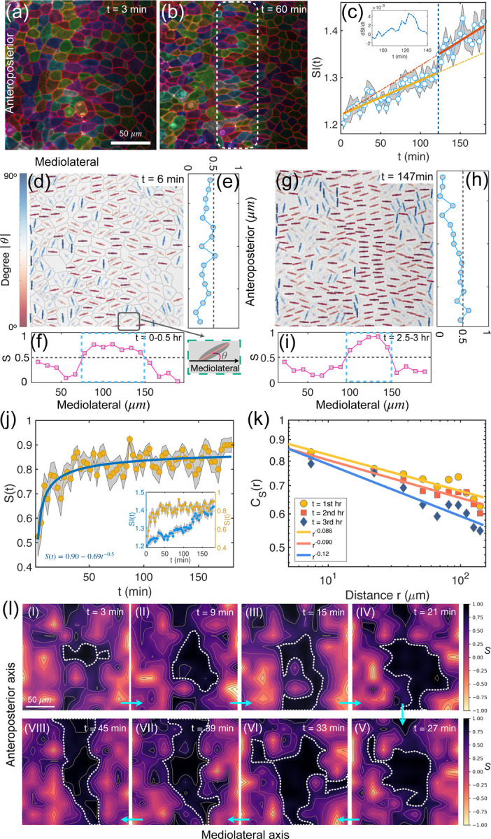
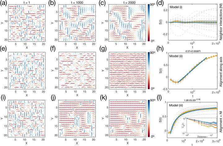
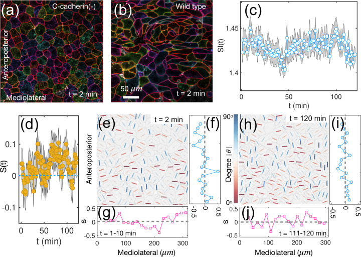
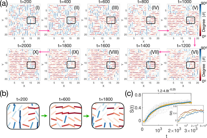
Cells undergo dramatic morphological changes during embryogenesis, yet how these changes affect the formation of ordered tissues remains elusive. Here, we show that a phase transition leading to the formation of a nematic liquid crystal state during gastrulation in the development of embryos of fish, frogs, and fruit flies occurs by a common mechanism despite substantial differences between these evolutionarily distant animals. Importantly, nematic order forms early before any discernible changes in the shapes of cells. All three species exhibit similar propagation of the nematic phase, reminiscent of nucleation and growth mechanisms. The spatial correlations in the nematic phase in the notochord region are long-ranged and follow a similar power-law decay ( $y~x^{-\alpha }$ ) with $\alpha$ less than unity, indicating a common underlying physical mechanism. To explain the common physical mechanism, we created a theoretical model that not only explains the experimental observations but also predicts that the nematic phase should be disrupted upon loss of planar cell polarity (frog), cell adhesion (frog), and notochord boundary formation (zebrafish). Gene knockdown or mutational studies confirm the theoretical predictions. The combination of experiments and theory provides a unified framework for understanding the potentially universal features of metazoan embryogenesis, in the process shedding light on the advent of ordered structures during animal development.

Figure 1.. Nematic order during zebrafish convergent extension (CE).

(a)-(b) Snapshots of zebrafish tissue at different times. The dashed rectangle in (b) shows the notochord location. The color associated with each cell is for illustration. (c) Temporal evolution of the shape index $SI\left(t\right)$ of cells in the notochord region shown in (b). The orange and red lines are linear fits ($SI\left(t\right)=7\times {10}^{-4}t+1.22,{10}^{-3}t+1.22$) with open circles (mean values), separated by the blue dashed line, where a jump in $SI\left(t\right)$ occurs (see the inset for the derivative of $SI\left(t\right)$). The shaded area indicates the standard error of mean (SEM). $n\approx 60$ cells from Video I. (d) Cell orientation, defined by the angle, $\theta$, between the long axis of cells (see the short lines) and the horizontal (mediolateral) axis of the embryo, (the inset at the bottom right of (d)) at $t=6min$. The short lines are color coded by the $\left|\theta \right|$ value (a key is shown to the left of panel $d$). (e)-(f) The nematic order parameter, $S$, as a function of the cell position along the anteroposterior or mediolateral axis. Each curve is averaged over 10-time frames spanning 30 minutes. (g)-(i) Same as (d-f) except at later timepoints of CE. (j) Time dependent changes in $S\left(t\right)$ of cells in the notochord region identified in (b). The solid line is a power-law fit ($S\left(t\right)=0.9-0.69t^{-0.53}$) with circles being the mean values. The shaded area shows the SEM. The inset shows the $SI\left(t\right)$ and $S\left(t\right)$ in the same plot. (k) The spatial correlation, $C_S\left(r\right)$ (Eq. (2)), of cells in the notochord region at different times. The solid lines show a power-law decay. The functional forms of the decay are displayed in the figure. (l) (I)-(VIII) The spatial-temporal evolution of $\mathit{S}$ shows the propagation of the nematic order (see the black region enclosed by the white dotted line where $S>0.8$). Each figure in (I)-(VIII) is averaged over two successive time frames (3-minutes interval). The scale bar in (a) and (l) is $50\mu m$.

Figure 2.. Emergence of a nematic phase during Xenopus CE.

(a)-(b) Snapshots of Xenopus laevis tissue at different timepoints. (c) Time dependent changes in the shape index SI(t) of the notochord cells in the field of view. The orange and red lines are linear fits ($SI\left(t\right)=4.7\times {10}^{-4}t+\mathrm{1.59,6.1}\times {10}^{-4}t+1.6$) with open circles (mean values). The data at early and late timepoints are separated by a jump (blue dashed line, see also the inset for the derivative of $SI\left(t\right)$) in $SI\left(t\right)$ at $t=70min$. The open circles give the mean $SI$ values of all cells in the field of view at each time point. The shaded area shows the SEM. $n\approx 200$ cells from Video IV. (d) Cell orientation in Xenopus tissues early during CE. The short lines are color coded by the value of $\left|\theta \right|$ (defined in Fig. 1d.) (e)-(f) Nematic order parameter, $S$, as a function of the cell position along anteroposterior or mediolateral axis at an early timepoint. The two curves are obtained by averaging over 30 successive time frames spanning one hour. (g)-(i) Same as (d)-(f), except later. (j) Temporal evolution of the nematic order parameter $S$ of cells in the field of view. The solid line is a power-law fit (functions listed in the figure) with circles (mean values). The shaded area shows the SEM. The inset shows the $SI\left(t\right)$ and $S\left(t\right)$ in the same plot. (k) Spatial correlation, S, of notochord cells at different times. Solid lines are a power-law fits (functions listed in the figure) of the data at different times. (l) (I)-(VIII) Same as Fig.1(l), showing the propagation of the nematic order (see the black region enclosed by the white dotted line). Each figure in (I)-(VIII) is averaged over three successive time frames (2-minutes interval). The scale bar in (a) and (l) is $50\mu m$.

Figure 3.. Emergence of nematic order in Drosophila during CE.

(a)-(b) Representative snapshots of lateral views of the Drosophila germband. (c) Shape index $SI\left(t\right)$ and $S\left(t\right)$ as a function of time for cells located in the dashed rectangle in (b). Linear fits ($SI\left(t\right)=-1.5\times {10}^{-3}t+1.17,\left.4.4\times {10}^{-3}t+1.05\right)$ with open circles (mean values) at different times, shown in orange and red. A jump (blue dashed line, see also the inset for the derivative of $SI\left(t\right)$) occurs at $t=30min$. The shaded area shows the SEM. $n\approx 100$ cells from Video V. (d) Cell orientation is defined by the angle, $\theta$, between the long axis of cells (see the short lines) and the anteroposterior axis. The short lines are color coded by the value of $\left|\theta \right|$. (e)-(f) Orientational order parameter, $S$, as a function of the cell position along the dorsal-ventral, anteroposterior axis. The two curves are obtained by averaging over 10 successive time frames in five minutes. (g)-(i) Same as (d)-(f), except at later times. (j) Temporal evolution of the nematic order parameter $S$ of cells in the dashed rectangle in (b). The solid line is a power-law fit ($S\left(t\right)=\Sigma -\Gamma t^{-\beta }$, with functions listed in the figure) of the data with circles (mean values). The shaded area shows the SEM. The inset shows the $SI\left(t\right)$ and $S\left(t\right)$ in the same plot. (k) Spatial correlation of $S$ for cells in the dashed rectangle in (b) at different times. The solid lines are a power-law fit ($C_S\left(r\right)\propto r^{-\alpha }$, with functions listed in the figure) at different times. (l) (I)-(VIII) Same as Fig.1(l), it shows the propagation of the nematic order during Drosophila development (see the black region enclosed by the white dotted line). Each figure in (I)-(VIII) is averaged over three successive time frames. (m) Scaled order parameter $S$ as a function of the scaled time $t/t_0\left(t_0=1min\right)$ for three organisms: zebrafish, Xenopus, and Drosophila. (n) Same as (m), except for the scaled spatial correlation of $S$ over the scaled distance $r/r_0.r_0$, mean cell size, is taken by $10\mu m$ for zebrafish and Drosophila, and $20\mu m$ for Xenopus. The same symbol but in different colors represents data taken at different times for the same organism. The inset is a zoom-in view of the dashed box. The scale bar in (a) and (l) is $20\mu m$.

Figure 4.. Models for nematic order formation.

(a)-(d) Results from model (i) (Materials and Methods), where each cell orientation ($\theta$) is influenced only by four neighbors. (a)-(c) Cell orientation at different times $t$. The parameter $𝒜=2.5\times {10}^{-3}$. (d) Time dependent changes in $S$ for all cells in (a). Each curve in gray represents one realization. Data in the brown dot is the mean value averaged over 20 trajectories. The shaded area shows the SEM. The solid line in navy blue corresponds to $S=0$. (e)-(h) Results from model (ii), where each cell orientation is influenced only by a global field, leading alignment along the $X$-axis independently. The navy-blue line in ($h$) is a linear function, listed at the top of the figure. The parameter $ℬ=1\times {10}^{-3}$. (i)-(l) Results from model (iii), Eq. (6). Navy blue line in (l) shows a power-law behavior with the function listed at the top of the figure. The values of $𝒜$ and $ℬ$ are 2.5×10⁻³, 1×10⁻³, respectively. The inset in (l) shows the spatial correlation, $C_S\left(r\right)$, of cells at different times from simulations. The solid lines show the power-law decay.

Figure 5.. Reduced nematic order in PCP mutant Xenopus.

(a)-(b) Two representative images of PCP-protein knockdown Xenopus tissue. (c) Orientation of cells in Xenopus tissue (PCP-) at an early timepoint. The short lines are color coded by the value of $|\theta \mid$. (d)-(e) Nematic order parameter, $S$, as a function of the cell position along the anteroposterior, mediolateral axis. Each curve is averaged over thirty successive time frames spanning 1 hour. (f)-(h) Same as (c)-(e), except at later timepoints. (i), (j) Dependence of $SI\left(t\right)$ and the nematic order parameter $S\left(t\right)$ as a function of t in Xenopus tissue with PCP protein knockdown. Open circles show the mean values, and the shaded area indicates the SEM. $n\approx 200$ cells from Video VI.

Figure 6.. Reduced nematic order in C-cadherin mutant Xenopus.

(a)-(b) Two representative snapshots of C-cadherin knockdown or wild-type Xenopus tissue. (c), (d) Dependence of $SI\left(t\right)$ and the nematic order parameter $S\left(t\right)$ as a function of $t$ in Xenopus tissue with $C$-cadherin knockdown. Open circles show the mean values, and the shaded area indicates the SEM. $n\approx 200$ cells from Video VII. (e) Orientation of cells in Xenopus tissue ($C$-cadherin-) at an early timepoint. The short lines are color coded by the value of $\left|\theta \right|$. (f)-(g) Nematic order parameter, $S$, as a function of the cell position along the anteroposterior, mediolateral axis. Each curve is averaged over ten successive time frames spanning 10 minutes. (h)-(j) Same as (e)-(g), except at later timepoints.

Figure 7.. Effects in C-cadherin mosaic mutants.

(a)-(b) Images of Xenopus tissue with c-cadherin mosaic mutant at $t=10s$ (a) and $t=130min$ (b). The cells labeled in green (red) are c-cadherin knock down (wild-type). (c)-(d) Cell orientation corresponds to the two snapshots in (a)-(b). The short lines are color coded by the angle $\left(\right|\theta \left|\right)$ between the long axis of cells and the horizontal axis of the tissue. (e)-(f) The nematic order parameter, $S$, as a function of the cell position along the anteroposterior or mediolateral axis. Each curve is averaged over 10-time frames. A clear jump in the value of $S$ is found along the mediolateral axis, where mutant and wild-type cells segregate clearly. (g)-(h) Temporal evolution of the shape index $SI\left(t\right)$ for cells on the left (mutant-type) or right (wild-type) region of the tissue. (i)-(j) Time dependent changes in $S\left(t\right)$ of cells on the left or right region as in (g)-(h). The differences between the mutant and the wild type are dramatic.

Figure 8.. Collapse of nematic order in spt mutant zebrafish.

(a)-(b) Two representative snapshots of zebrafish tissue in spt-mutant or wild type. The dashed rectangle shows cells around the middle line. (c)-(d) $SI\left(t\right)$ and $S\left(t\right)$ as a function of $t$ for the spt-mutant cells in the field of view. The mean (SEM) is shown in open circles (shaded area). $n\approx 300$ cells from Video VIII. (e) Cell orientation ($\theta$) in zebrafish spt-mutant early times. (f)-(g) The orientational order parameter, $S$, as a function of the cell position along the anteroposterior, mediolateral axis at early times. Lines are averaged over ten successive time frames spanning 30 minutes. (h)-(j) Same as (e)-(g), except at later times. The scale bar in (b) and (l) is $50\mu m$.

Figure 9.. Computational results for the mutant Xenopus and zebrafish tissues.

(a)-(c) The cell orientation ($\theta$) in Xenopus mutants at different times. The short lines are color coded by the value of $\left|\theta \right|$. The parameter values are: $𝒜={10}^{-6}$, and $ℬ=3\times {10}^{-4}$ (see Eq. (7) in the main text). Time is measured in simulation steps. (d) The temporal evolution of the nematic order parameter $S\left(t\right)$ of cells in mutant Xenopus tissues. Each curve in gray represents a single trajectory. Data in the brown dot is the mean value averaged over 20 trajectories. The shaded area shows the SEM. (e)-(h) Similar to (a)-(d) for zebrafish mutant tissues. The parameter values are: $𝒜=2.5\times {10}^{-3}$, and $ℬ=1\times {10}^{-3}$ for $t<1000$, while $ℬ=-1\times {10}^{-3}$ for $t\ge 1000$.

Figure 10.. Nematic order in the presence of noise.

(a) Cell orientation at different times $t$. The parameters $A$ and $B$ are the same as used in model (iii) in Fig. 4(i)–(l) but with an additional term representing the noise, $C\zeta \left(t\right)$. $\zeta$ is white noise with zero mean and variance, $⟨\zeta \left(t\right)\zeta \left(t^{\prime }\right)⟩=\delta \left(t-t^{\prime }\right)$. The value of $C$ is 5×10⁻². Like Fig. 4(i)–(k), cells become orientated along the horizontal axis as time $t$ increases. Certain regions (see the one enclosed by the black boxes in each figure for an example) can change from disorder to order or vice versa due to noise-induced fluctuations. (b) A zoomed in view of the region in the boxes for (a) to showing the transitions between the ordered and disordered phases. (c) Time dependent changes in $S$ for all cells in (a). Each curve in gray represents one realization. Data in the brown dot is the mean value averaged over 20 trajectories. The shaded area shows the SEM. Navy blue line shows a power-law behavior with the function listed at the top of the figure. The inset shows several representative individual trajectories from the main figure, showing a fluctuation of $S$ over time.

References

1. Shindo A. Models of convergent extension during morphogenesis. Wiley Interdiscip. Rev. Dev. Biol. 7, e293 (2018). - PMC - PubMed
1. Walck-Shannon E., & Hardin J. Cell intercalation from top to bottom. Nat. Rev. Mol. Cell Biol. 15, 34–48 (2014). - PMC - PubMed
1. Huebner R. J. & Wallingford J. B. Coming to consensus: a unifying model emerges for convergent extension. Dev. Cell 46, 389–396 (2018). - PMC - PubMed
1. Williams M. L. & Solnica-Krezel L. Cellular and molecular mechanisms of convergence and extension in zebrafish. Curr. Top. Dev. Biol. 136, 377–407 (2020). - PMC - PubMed
1. Keller R., & Sutherland A. Convergent extension in the amphibian, Xenopus laevis. Curr. Top. Dev. Biol. 136, 271–317 (2020). - PMC - PubMed
Publication types
LinkOut - more resources