pyRBDome: a comprehensive computational platform for enhancing RNA-binding proteome data

Abstract

High-throughput proteomics approaches have revolutionised the identification of RNA-binding proteins (RBPome) and RNA-binding sequences (RBDome) across organisms. Yet, the extent of noise, including false positives, associated with these methodologies, is difficult to quantify as experimental approaches for validating the results are generally low throughput. To address this, we introduce pyRBDome, a pipeline for enhancing RNA-binding proteome data in silico. It aligns the experimental results with RNA-binding site (RBS) predictions from distinct machine-learning tools and integrates high-resolution structural data when available. Its statistical evaluation of RBDome data enables quick identification of likely genuine RNA-binders in experimental datasets. Furthermore, by leveraging the pyRBDome results, we have enhanced the sensitivity and specificity of RBS detection through training new ensemble machine-learning models. pyRBDome analysis of a human RBDome dataset, compared with known structural data, revealed that although UV-cross-linked amino acids were more likely to contain predicted RBSs, they infrequently bind RNA in high-resolution structures. This discrepancy underscores the limitations of structural data as benchmarks, positioning pyRBDome as a valuable alternative for increasing confidence in RBDome datasets.

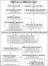
Figure 1.. Schematic representation of the pyRBDome pipeline.

To run the pipeline, the user needs to provide a table, with the same column names as shown in the table, that includes the UniProt identifier (ID), the name of the protein, cross-linked amino acids (if available), cross-linked peptides (if available), and the location of the cross-linked amino acid in the corresponding cross-linked peptide sequence. This table is then used to download structural information from rcsb.org or from AlphaFold2. The protein structures (in PDB files) are then submitted to various web servers that predict ligand-binding sites on the protein. The protein sequences are extracted from the PDB files and submitted to prediction algorithms that use sequence-based information to predict RNA-binding sites (RBSs). Domain information is also extracted from the protein sequences, using the InterProScan tool. Once all the predictions have been completed, the pipeline gathers all the data by collating the results in a SQLite database (see Fig S6 for an example of such a table). This is then fed to our XGBoost ensemble model to predict RBS, with the aim of further enhancing the detection of RBSs. The resulting data are then highlighted within the provided cross-linked peptide sequence. Moreover, statistical analyses are performed to determine whether cross-linked peptides/amino acids are enriched for predicted RBSs.

Figure S1.. Schematic representation of the complete pyRBDome pipeline.

For a detailed description, please see the main text and the Materials and Methods section. Briefly, to start running the pipeline, a CSV file containing UniProt IDs is a minimum requirement. Information about cross-linked peptide and amino acid sequences can also be included. An example of an input file can be found on our Git repository (https://git.ecdf.ed.ac.uk/sgrannem/pyRBDome_Notebooks/-/blob/main/pyRBDome_analyses/RBSID_human_data.xlsx). Each discrete analysis step in the pipeline is indicated with boxes. The names ending with. ipynb indicate the names of the Jupyter notebooks that are used in each step of the analysis.

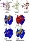
Figure 2.. Ground truth analysis results for the Streptococcus pyogenes Cas9 protein.

Shown is a surface representation of the structure of the spCas9 protein in complex with cocrystallised RNA and DNA (orange colour), obtained from rcsb.org (PDB 4un3 [Anders et al, 2014]). (A, B, C) Results of the protein–ligand interaction profiler analysis (Adasme et al, 2021) on the spCas9-RNA interactions. Shown are the results for all the RNA-binding residues (A), the amino acids that form hydrogen bonds with RNA (B), and those that form salt bridges (C). Blue amino acids indicate those that do not bind RNA directly. Red amino acids indicate those that do. (D) Highlighting amino acids that are in proximity to RNA in the spCas9-RNA complex. To generate the GT-Distance ground truth dataset, we considered amino acids that are within 4.2 Å of RNA in the available structures as RNA-binding. Those amino acids closest to RNA are highlighted in red, whereas those >4.2 Å from RNA are highlighted in blue.

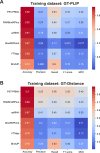
Figure S2.. Performance metrics for protein–RNA interaction predictors employed by pyRBDome.

(A, B) These heatmaps represent the comparative analysis of tools used for predicting amino acid–RNA (PST-PRNA, aaRNA, RNABindRPlus, DisoRDPbind, and BindUP) or small molecule interaction sites (FTMap). For these analyses we used the GT-PLIP (A) or GT-Distance (B) ground truth datasets. TP, true positives; FP, false positives; TN, true negatives; FN, false negatives. Five key performance metrics were calculated, with higher values indicating higher performance: accuracy: the proportion of true results (both true positives and true negatives) among the total number examined (TP + TN)/(TP + FP + FN + TN). Precision: proportion of true positives among the total predicted as positive (TP/[TP + FP]). Recall (sensitivity): proportion of positives correctly identified (TP/[TP + FN]). F1 score: harmonic mean of precision and recall: (2 × [Precision × Recall]/[Precision + Recall]). Matthews correlation coefficient (MCC): a measure of the quality of the classifications that takes into consideration all four confusion matrix categories (TP, FP, FN, and TN): ([TP × TN − FP × FN]/sqrt [TP + FP] × [TP + FN] × [TN + FP] × [TN + FN]).

Figure 3.. pyRBDome analysis results for the spCas9 protein.

(A) Shown is the structure of the RNA and DNA molecules within the structure, as well as the individual spCas9 protein domains detected by InterProScan (Jones et al, 2014). (B) Same as in (A) but now with the location of cross-linked peptides within the structure. (C) Same as in (B) but now with the location of the cross-linked amino acids (shown as surface, red colour). (D, E, F, G). Examples of prediction results from various tools employed by pyRBDome. Shown is a surface representation of the spCas9 protein, with nucleic acids shown in orange. Accompanying colour bars represent the RNA-binding propensities, correlating specific colours with their respective values.

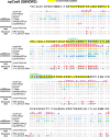
Figure S3.. Overview of the spCas9 pyRBDome prediction results in the protein sequence.

Domains identified in the protein are outlined with ovals. Cross-linked peptides are highlighted in yellow. The score bar represents the RNA-binding probabilities for the amino acid residues as determined by our XGBoost model using the combined prediction results. The additional rows show results from various predictors (PST-PRNA, BindUP, FTMap, RNABindRPlus, and DisoRDPbind). Here, the coloured acid residues indicate those with values at or above the recommended probability/score thresholds. The cross-linked amino acids identified by RBS-ID are indicated in the experimental data track in pink. The ground truth analysis results for spCas9 are also presented: RNA-binding track: red-coloured residues bind RNA in the Cas9-RNA structure. ≤ 4.2 A from RNA: the dark grey-coloured residues are amino acids positioned within 4.2 Å of RNA in the spCas9 structure analysed (PDB 4un3 [Anders et al, 2014]).

Figure S4.. Analysis of amino acid and domain cross-linking preferences in RBD-ID data.

(A) Counts (black bars) and frequency (blue bars) of cross-linked amino acids. Frequency is calculated by dividing the total counts of each amino acid observed in the cross-linking data by the total occurrence of that amino acid in the protein sequences of the analysed proteins. (B) Same as in (A) but now for the chemical properties of the amino acids. Categories: L, aliphatic; R, aromatic; C, acidic; B, basic; H, hydroxylic; S, sulphur-containing; M, amidic. (C) Histogram displaying the total number of times a cross-linking peptide was detected in specific protein domains.

Figure 4.. Cross-linked peptides are enriched for tripeptides containing aromatic and positively charged amino acids flanked by aliphatic residues.

(A) Tripeptide motifs detected in RNA-binding regions (amino acids within 4.2 Å from RNA) from known RNA-binding proteins. (B) Tripeptide motifs enriched in the RBS-ID cross-linked peptides. (A, C) Enriched chemical properties of tripeptide sequences detected in the ground truth data described in (A). (D) as in (B) but now showing the chemical properties. Categories: L, aliphatic; R, aromatic; C, acidic; B, basic; H, hydroxylic; S, sulphur-containing; M, amidic. P-values were calculated using the Fisher exact test and corrected for multiple testing using the Benjamini–Hochberg procedure.

Figure 5.. Insights into RNA-binding interfaces in protein domains through aggregated amino acid UV cross-linking data.

(A) Superimposed peptide sequences mapped to RNA recognition motif (RRM) domains in proteins identified in the RBS-ID dataset. These sequences were aligned on available structural models of RRM domain–containing proteins. The various α- and β-secondary structural elements within the RRM domains are also indicated. (B) As in (A), but with the side chains of UV cross-linking sites within the domains highlighted as yellow sticks. The white cloud represents the surface area of the RRM domains. (C) Number of UV cross-links detected in all superimposed RRM domains (y-axis), correlating to their specific positions within the domain (x-axis). Below the x-axis, the consensus secondary structure for RRM domains is depicted for reference.

Figure S5.. Insights into RNA-binding interfaces in protein domains through aggregated amino acid UV cross-linking data that can only be generated with data containing many cross-links.

This figure presents the findings for proteins with KH domains. (A) Superimposed peptide sequences mapped to RNA recognition motif (RRM) domains in proteins identified in the RBS-ID dataset. These sequences were aligned on available structural models of RRM domain–containing proteins. The various a and b secondary structural elements within the RRM domains are also indicated. Side chains of UV–cross-linked amino acids within the domains are highlighted as yellow sticks. The white cloud represents the surface area of the RRM domains. (B) Number of UV cross-links detected in all KH domains at specific positions (y-axis), correlating to their specific positions within the domain (x-axis). Below the x-axis, the consensus secondary structure for KH domains is depicted for reference. GXXG (green) and “variable loop” indicate key regions involved in RNA recognition.

Figure S6.. Schematic representation of how the data from the individual prediction results are used to train the XGBoost models.

Data from those tools that provide RNA-binding propensity are directly fed to XGBoost. The x and y characters indicate the experimental and ground truth data, respectively. Values for BindUP, with 10 or higher indicating an RNA-binding site, were normalised to values between 0 and 1. To enable analysis of the FTMap docking results with XGBoost, we calculated the minimum distance of each amino acid in the PDB file to docked ligands. These values were then converted to values between 0 and 1, with the highest value indicating a high ligand-binding score. These values were then used to train XGBoost models. 80% of the GT-PLIP and GT-Distance datasets were used for training purposes and 20% for testing. For the analyses shown in Fig 10, 50% of the data were used for training and 50% for testing. Once the parameters for the models were optimised, they were used to predict RNA-binding amino acids for the proteins in the RBS-ID dataset (column “predictions”). These values represented RNA-binding probabilities. All the analysis results are provided in Tables S4 and S5.

Figure 6.. Assessment of XGBoost models trained on prediction models.

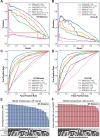
(A, B) Precision–recall curves for the various XGBoost prediction models trained on the GT-Distance (A) and GT-PLIP (B) ground truth datasets using the predictions from either the individual tools or all predictions combined. The AP score for each model is indicated in the legend (e.g., aaRNA AP = 0.44). (C, D) Receiver operating characteristic curves for the same prediction models using the GT-Distance (C) and GT-PLIP ground truth datasets (D), with AUC scores provided in the legend. (E, F) Bar graph comparing the AP (E) and AUC (F) scores across different XGBoost models for the GT-Distance training dataset. The XGBoost models were trained on results from different combinations of prediction algorithms. The heatmap below the bar plot indicates what model combinations were used for training and testing the model.

Figure S7.. Evaluation of predictor significance in XGBoost model efficacy.

(A) Relative importance of different predictors as determined by our XGBoost model. The importance is measured based on how much each predictor contributes to the accuracy of the model. The predictors are listed on the y-axis and their corresponding importance on the x-axis. (B) Normalised feature importance of each predictor against its total mean value from the predictions. The x-axis represents the normalised importance assigned by the XGBoost model, whereas the y-axis shows the mean value of the prediction results from each tool. The mean is calculated using the accumulation of the impurity decrease within each tree, which is essentially the average of how much the decision made in each tree of the XGBoost model helps to improve the decision-making across all trees.

Figure S8.. PNPase AlphaFold2 model similarity to published crystal structures.

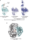
(A) Crystal structure of the C. crescentus PNPase trimer bound with RNA (PDB ID 4AM3 [Hardwick et al, 2012]). Noted are the positions of the cocrystallised RNA fragment and the RNA-binding GSGG loop. (B) Crystal structure of the C. crescentus PNPase monomer in complex with RNA. Highlighted are the cocrystallised RNA fragment and the RNA-binding GSGG loop. In addition, the crystal structure of the S. aureus PNPase active site alongside the AlphaFold2 model is presented. Below the models, the root-mean-square deviation values for the various model comparisons are provided.

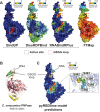
Figure 7.. pyRBDome detects known RNA-binding regions in S. aureus polynucleotide phosphorylase (PNPase).

(A) Results from prediction algorithms on the surface representation of a PNPase monomer. The colours for BindUP, DisoRDPbind, and RNABindRPlus results indicate RNA-binding probabilities, with cooler shades (blue) suggesting lower and warmer shades (red) indicating a higher RNA-binding likelihood. For the FTMap results, warmer red shades signify shorter distances to docked molecules. The active site of the nuclease is marked with a square box. The GSGG loop is marked with a red square box. Blue colours represent amino acids with low RNA-binding prediction scores (BindUP, DisoRDPbind, or RNABindRPlus), whereas red colours indicate amino acids with high RNA-binding prediction scores. For the FTMap data, the blue-to-red colour gradient denotes decreasing distance to docked small molecules, with red indicating distances of ≤2 Å and blue indicating distances of >4.2 Å. Accompanying colour bars represent the RNA-binding propensities, correlating specific colours with their respective values. (B) Crystal structure of PNPase from C. crescentus, in complex with RNA, PDB ID 4AM3 (Hardwick et al, 2012). The RNase PH-like domains, coloured in dark and light pink, are linked by a helical domain, coloured in yellow. The KH domain (green) interacts with the RNA of the structure through the GSGG loop (red). The S1 domain is absent from this crystal structure. (C) Structural alignment of the RNA from structure 4AM3 on the PNPase AlphaFold2 model with results from XGBoost model predictions trained on the prediction results from all algorithms. Catalytic residues are displayed as spheres and are highlighted in an enlarged view of the active site region.

Figure 8.. Limited concordance between UV cross-linking data and protein–RNA structures.

(A) Cumulative distribution of distances for cross-linked amino acids (yellow), randomly shuffled amino acids (blue), and the total pool of amino acids (green), in comparison with established RNA-binding amino acids determined by protein–ligand interaction profiler. P-values, calculated using the KS test, indicate significant differences between groups. The 4.2 Å threshold, indicated by the dashed vertical line, is used to determine the proximity required for hydrogen bonding. (B) Similar to (A), this analysis plots the cumulative distances of cross-linked, randomly selected, and all amino acids within the studied RNA-binding proteins, relative to their proximity to RNA. The KS test was also employed here to calculate P-values. (C) Amino acids that form π-stacking interactions are often cross-linked to RNA. The pie chart displays the percentages of each cross-linked amino acid involved in different types of interactions: hydrogen-bonding (H-bond), π-stacking, π-cation, salt bridge, and hydrophobic interactions, as identified by protein–ligand interaction profiler. These percentages were calculated by dividing the number of a specific type of interaction by the total number of such interactions detected in the analysed structures. (D) Counts of cross-linked amino acids involved in p-stacking interactions. Y = tyrosine; H = histidine; F = phenylalanine; and W = tryptophan.

Figure 9.. Cross-linked peptides as reliable proxies for RNA-binding sites.

(A) Violin plots showing the distribution of RNA-binding probabilities as determined by our XGBoost model for cross-linked, randomly shuffled amino acids, and all available amino acids within the analysed RNA-binding proteins. (B) Distribution of the highest RNA-binding probability score (determined by our XGBoost models) detected in cross-linked peptide sequences. Control datasets included randomly generated peptides with the same length distribution, and peptide libraries generated in silico by Lys-C or trypsin digestion of the RNA-binding proteins analysed here. (C) As in (B), but now for the average RNA-binding probabilities calculated for each cross-linked peptide. P-values, calculated using a two-sided Mann–Whitney–Wilcoxon test with the Bonferroni correction, indicate significant differences between groups, as shown above each comparison. The violins represent density estimations of the distances, with wider sections indicating a higher frequency of distances. The white dot in the centre of each violin plot denotes the median distance, and the thick lines within the violins represent the interquartile ranges.

Figure S9.. UV–cross-linked peptides in RBS-ID data are enriched for RNA- and small molecule binding sites or are more likely to be in closer proximity.

(A) This panel displays the distribution of distances to RNABindRPlus predicted RBSs identified in cross-linked peptide sequences. Comparative control datasets include randomly generated peptides matching the length distribution and peptide libraries produced in silico through Lys-C or trypsin digestion of the analysed RNA-binding proteins. P-values were calculated using a two-sided Mann–Whitney U test with the Bonferroni correction, highlighting significant differences between the groups as denoted above each comparison. The violins depict density estimates of the distances, where broader sections suggest a higher frequency of amino acids at specific distances. The white dot at the centre of each violin plot signifies the median distance, whereas the thick bars within the violins indicate the interquartile ranges. (B) As (A) but presenting results for aaRNA predictions. (C) As (A) but illustrating the results for distances to FTMap-docked small molecules.

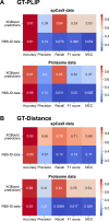
Figure 10.. Performance metrics used when comparing the RBS-ID cross-linked amino acids to the XGBoost predictions and ground truth datasets.

Colours closer to red indicate high performance, whereas colours closer to blue indicate poor performance. (A) Comparing the XGBoost predictions with the spCas9 and proteome RBS-ID cross-linking data using GT-protein–ligand interaction profiler data generated from published protein–RNA structures. (B) Same as in (A) but now considering amino acids that are within 4.2 Å from RNA as RNA-binding residues. Explanation of the performance metrics: accuracy: the frequency of model predictions that are correct. Note that mostly the non–RNA-binding amino acid residues are correctly predicted. Precision: measures what fraction of the items predicted as positive by RBS-ID and XGBoost are also positive in the ground truth datasets. Recall: measures what fraction of the positive items in the ground truth datasets were identified correctly by RBS-ID and our XGBoost model. F1 score: the harmonic mean of precision and recall. The F1 score reaches its best value at 1 (perfect precision and recall) and worst at 0. MCC: the Matthews correlation coefficient considers true and false positives and negatives and returns a value between −1 and +1, where +1 indicates perfect prediction, 0 indicates random prediction, and −1 indicates total disagreement between prediction and observation.

References

1. Adasme MF, Linnemann KL, Bolz SN, Kaiser F, Salentin S, Haupt VJ, Schroeder M (2021) PLIP 2021: Expanding the scope of the protein-ligand interaction profiler to DNA and RNA. Nucleic Acids Res 49: W530–W534. 10.1093/nar/gkab294 - DOI - PMC - PubMed
1. Akiba T, Sano S, Yanase T, Ohta T, Koyama M (2019) Optuna: A next-generation hyperparameter optimization framework. arXiv. 10.48550/arXiv.1907.10902 (Preprint posted July 25, 2019). - DOI
1. Anders C, Niewoehner O, Duerst A, Jinek M (2014) Structural basis of PAM-dependent target DNA recognition by the Cas9 endonuclease. Nature 513: 569–573. 10.1038/nature13579 - DOI - PMC - PubMed
1. Arora V, Sanguinetti G (2022. a) Challenges for machine learning in RNA-protein interaction prediction. Stat Appl Genet Mol Biol 21. 10.1515/sagmb-2021-0087 - DOI - PubMed
1. Arora V, Sanguinetti G (2022. b) De novo prediction of RNA–protein interactions with graph neural networks. RNA 28: 1469–1480. 10.1261/rna.079365.122 - DOI - PMC - PubMed
Associated data
LinkOut - more resources