. 2024 May 15;11(5):231511.
doi: 10.1098/rsos.231511. eCollection 2024 May.

Collective order and group structure of shoaling fish subject to differing risk-level treatments with a sympatric predator

Affiliations

Collective order and group structure of shoaling fish subject to differing risk-level treatments with a sympatric predator

Timothy M Schaerf et al. R Soc Open Sci. .

Abstract

It is imperative for individuals to exhibit flexible behaviour according to ecological context, such as available resources or predation threat. Manipulative studies on responses to threat often focus on behaviour in the presence of a single indicator for the potential of predation, whereas in the wild perception of threat will probably be more nuanced. Here, we examine the collective behaviour of eastern mosquitofish (Gambusia holbrooki) subject to five differing threat scenarios relating to the presence and hunger state of a jade perch (Scortum barcoo). Across threat scenarios, groups exhibit unique behavioural profiles that differ in the durations that particular collective states are maintained, the probability of transitions between states, the size and duration of persistence of spatially defined subgroups, and the patterns of collective order of these subgroups. Under the greatest level of threat, subgroups of consistent membership persist for longer durations. Group-level behaviours, and their differences, are interconnected with differences in estimates of the underlying rules of interaction thought to govern collective motion. The responses of the group are shown to be specific to the details of a potential threat, rather than a binary response to the presence or absence of some form of threat.

Keywords: Gambusia holbrooki; collective movement; group order; predator–prey; rules of interaction; threat.


Conflict of interest statement

We declare we have no competing interests.

Figures

Schematic representation of experimental arena used across risk gradient treatments. The arena consisted of three primary zones as represented by a central open water zone
Figure 1.
Schematic representation of experimental arena used across risk gradient treatments. The arena consisted of three primary zones as represented by a central open water zone (a) flanked by two shallow platform zones (b) on either side. When the predator (S. barcoo) was present visually (T3–T5) it was located in the central zone. Across treatments, mosquitofish (G. holbrooki) could move across the three zones (a and b) freely but were prevented from reaching the outermost areas (c) beyond the platforms by an opaque partition. In the predator cues treatment (T2), the predator was located in one of these two outermost areas on either side of the platform zones and water (containing cues) was mixed with the experimental observation area. The width of the tank was 30 cm, and the tank was filled to a depth of 17 cm with aged, conditioned tap water. The central zone (a) and each of the platform regions (b) were 22 cm long. The heights of the platforms were 15 cm, such that the depth of water was 2 cm above the platforms. The outermost areas (c) were 27 cm in length. (Adapted from fig. 1 in [47].)
Empirical cumulative density functions (a) and relative frequency histograms (b–f) of the mean median subgroup size observed for each treatment. Each curve
Figure 2.
Empirical cumulative density functions (a) and relative frequency histograms (b–f) of the mean median subgroup size observed for each treatment. Each curve in (a) shows the probability of the mean median subgroup size occupied by individuals being less than or equal to that on the horizontal axis for T1 (control—black), T2 (predator cue—green), T3 (predator fed with pellets—blue), T4 (predator fed with mosquitofish—magenta) and T5 (hungry predator—red) treatments. For the histograms (b–f), the number of trials was as follows: (T1) control, n = 13; (T2) predator cues, n = 10; (T3) pellet-fed predator, n = 12; (T4) mosquitofish-fed predator, n = 11; and (T5) hungry predator, n = 13.
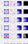
Force-map estimates for individual changes in speed (a, d, g, j, m) and direction of motion (b, e, h, k, n) as a function of the relative coordinates of neighbouring fish, and the relative frequencies of collective order parameter pairs (c, f, i, l, o)
Figure 3.
Force-map estimates for individual changes in speed (a, d, g, j, m) and direction of motion (b, e, h, k, n) as a function of the relative coordinates of neighbouring fish, and the relative frequencies of collective order parameter pairs (c, f, i, l, o). Treatments increase from T1 to T5 moving down the rows in the above plots. In the left and middle columns, the focal individual is located at the origin (0, 0), with its direction of motion parallel to the positive x-axis (travelling from left to right). The position and direction of motion of the focal individual is illustrated by a black arrow in the leftmost and middle columns. Positive changes in speed are rendered in red, and negative changes in speed in blue in the left column; the colour scale for the change in speed plots has been truncated at ±40 mm s−2, such that the darkest colours indicate speed changes of at least 40 mm s−2 in magnitude. Positive changes in direction of motion (corresponding to anticlockwise or left turns by the focal individual) are rendered in red, and negative changes in direction (corresponding to clockwise or right turns) are rendered in blue in the middle column. In the relative frequency plots in the right column, regions in parameter spacing corresponding to milling (M), parallel motion (P) and swarming (S) are demarcated by red dashed lines. Any (Or,Op) pairs outside the milling, parallel motion and swarming regions were treated as being representative of composite motion. Black regions in the plots outside the main coloured regions indicate zero relative frequency. Arrows superimposed on the relative frequency plots indicate the mean direction of change in parameter space (an estimate for the direction of dOp/dOr ).
Total proportions of time spent in collective states automatically classified as milling (M), parallel motion (P), swarming (S) or composite motion
Figure 4.
Total proportions of time spent in collective states automatically classified as milling (M), parallel motion (P), swarming (S) or composite motion (c). (a) Illustrates the total proportion of time spent in each state using data aggregated across all observations within each treatment. The boxplots, (b) to (e), were derived from the proportion of time spent in each state for each experimental trial.
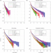
Log-survival curves, ln S, for unbroken durations spent by the whole group in each collective state, collated by the form of the collective state (a) milling, (b) parallel motion, (c) swarming and (d) composite motion)
Figure 5.
Log-survival curves, ln S, for unbroken durations spent by the whole group in each collective state, collated by the form of the collective state ((a) milling, (b) parallel motion, (c) swarming and (d) composite motion). 95% confidence intervals for the estimated survival curves are illustrated by shaded regions, bounded by dotted lines. By treatment, the curves correspond to T1 (black curves), T2 (green), T3 (blue), T4 (magenta) and T5 (red).
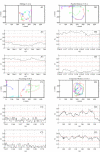
Smoothed individual tracks and associated order parameters for the longest duration instances of milling (a), swarming (b), parallel motion (c) and composite motion (d) in T1 (control)
Figure 6.
Smoothed individual tracks and associated order parameters for the longest duration instances of milling (A), swarming (B), parallel motion (C) and composite motion (D) in T1 (control). Along each track, each individual’s starting position is marked with a circle, and their position at the end of the group movement is marked with a square. The illustrated tracks were smoothed via a Savitzky–Golay filter (of span 5 and degree 2). Straight black lines on the panels illustrating the tracks represent the boundary of the experimental arena on the exterior, and also demarcate the central chasm region from the platforms to the left and right. Op and Or are the polarization and group angular momentum for the duration that the illustrated groups undertook each form of motion, plotted as a function of time in seconds. Electronic supplementary material, videos S1–S4 provide animations of the movements of the individuals shown in the static images of panels (A1), (B1), (C1) and (D1), respectively.
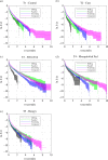
Log-survival curves, ln S, for unbroken durations spent by the whole group in each collective state, collated within the treatment (a) T1 (control), (b) T2 (cues), (c) T3 (pellet fed), (d) T4 (mosquitofish fed), (e) T5 (hungry predator)
Figure 7.
Log-survival curves, ln S, for unbroken durations spent by the whole group in each collective state, collated within the treatment (a) T1 (control), (b) T2 (cues), (c) T3 (pellet fed), (d) T4 (mosquitofish fed), (e) T5 (hungry predator). 95% confidence intervals for the estimated survival curves are illustrated by shaded regions, bounded by dotted lines. By state, the curves correspond to milling (black curves), parallel motion (green), swarming (blue) and composite motion (magenta).
Observed relative frequencies (probabilities) of transitions between collective states at each video frame/discrete time step of data. Arrows indicate the direction of each transition
Figure 8.
Observed relative frequencies (probabilities) of transitions between collective states at each video frame/discrete time step of data. Arrows indicate the direction of each transition, loops indicate no change in state, and the colour scale indicates the transition probability, ranging from 0 (dark blue) to 1 (dark red).
Log-survival functions of durations that subgroups of different sizes persisted within each treatment, with 95% confidence intervals (shaded regions)
Figure 9.
Log-survival functions of durations that subgroups of different sizes persisted within each treatment, with 95% confidence intervals (shaded regions), ((a) T1 (control), (b) T2 (cues), (c) T3 (pellet fed), (d) T4 (mosquitofish fed), (e) T5 (hungry predator)). Survival functions for subgroups of 1 are plotted in red, and survival functions for subgroups of size 8 are plotted in blue. Survival curves for all other subgroup sizes are plotted in black. The criteria for subgroup membership was based on subgroup members being within four body lengths of each other.
Log-survival functions of durations that subgroups of different sizes persisted across treatments, with 95% confidence intervals (shaded regions)
Figure 10.
Log-survival functions of durations that subgroups of different sizes persisted across treatments, with 95% confidence intervals (shaded regions). The survival curves are coloured as follows: T1 (control—black), T2 (predator cue—green), T3 (predator fed with pellets—blue), T4 (predator fed with mosquitofish—magenta) and T5 (hungry predator—red). Subgroup sizes range from 1 (a) to 8 (h)
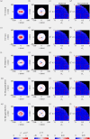
Local subgroup structure, alignment and collective order parameter summary for subgroups of 2. Each row corresponds to a different treatment, as indicated by the leftmost labels
Figure 11.
Local subgroup structure, alignment and collective order parameter summary for subgroups of 2. Each row corresponds to a different treatment, as indicated by the leftmost labels. The leftmost column (a,e,i,m,q) illustrates the relative frequency that mosquitofish occupied particular positions relative to the subgroup centroid, and the second column from the left (b,f,j,n,r) illustrates the direction of motion of subgroup members relative to that of the subgroup centroid, as a function of the relative positions of the fish. In each plot in the left two columns, the group centre is located at (0, 0), such that the direction of motion of the subgroup centre is parallel to the positive x-axis (the position and heading of the group centre is represented by small black arrows in the left two columns). In the relative alignment plots, blue colours indicate that individuals tended to be rotated clockwise relative to the positive x-axis and red colours indicate that individuals tended to be rotated anticlockwise relative to the positive x-axis. Note that the colour scale on the relative alignment plots has been truncated at ±20° to clarify the sense (clockwise or anticlockwise) of relatively small angular differences. The right two columns illustrate the relative frequency that particular order parameter pairs (Or, Op) , occurred across all observations for a given treatment, in preferred (third column from the left, (c,g,k,o,s)) and non-preferred (fourth column from the left, (d,h,l,p,t)) regions of the experimental aquaria; arrows in these plots indicate the average direction of dOp/dOr . For T1 and T2, the preferred zone (determined by the total time spent in each zone) was the central zone, whereas for T3, T4 and T5, the preferred zones were the platform regions. Conversely, the non-preferred zones were the platform regions for T1 and T2 groups, and the central zone for T3, T4 and T5.
Local subgroup structure, alignment and collective order parameter summary for subgroups of 8 (i.e. the entire group when all group members were relatively close to each other)
Figure 12.
Local subgroup structure, alignment and collective order parameter summary for subgroups of 8 (i.e. the entire group when all group members were relatively close to each other). The leftmost column (a,e,i,m,q) illustrates the relative frequency that mosquitofish occupied particular positions relative to the subgroup centroid, and the second column from the left (b,f,j,n,r) illustrates the direction of motion of subgroup members relative to that of the subgroup centroid, as a function of the relative positions of the fish. In each plot in the left two columns, the group centre is located at (0, 0), such that the direction of motion of the subgroup centre is parallel to the positive x-axis (the position and heading of the group centre is represented by small black arrows in the left two columns). In the relative alignment plots, blue colours indicate that individuals tended to be rotated clockwise relative to the positive x-axis and red colours indicate that individuals tended to be rotated anticlockwise relative to the positive x-axis. Note that the colour scale on the relative alignment plots has been truncated at ±20° to clarify the sense (clockwise or anticlockwise) of relatively small angular differences. The right two columns illustrate the relative frequency that particular order parameter pairs (Or, Op) , occurred across all observations for a given treatment, in preferred (third column from the left, (c,g,k,o,s)) and non-preferred (fourth column from the left, (d,h,l,p,t)) regions of the experimental aquaria; arrows in these plots indicate the average direction of dOp/dOr . For T1 and T2, the preferred zone (determined by the total time spent in each zone) was the central zone, whereas for T3, T4 and T5, the preferred zones were the platform regions. Conversely, the non-preferred zones were the platform regions for T1 and T2 groups, and the central zone for T3, T4 and T5.

References

    1. Ward AJW, Webster MM. 2016. Sociality: the behaviour of group-living animals. Cham, Switzerland: Springer. (10.1007/978-3-319-28585-6) - DOI
    1. Seeley TD. 2010. Honeybee democracy. Princeton, NJ: Princeton University Press. (10.1515/9781400835959) - DOI
    1. Ward AJW, Herbert-Read JE, Sumpter DJT, Krause J. 2011. Fast and accurate decisions through collective vigilance in fish shoals. Proc. Natl. Acad. Sci. USA 108 , 2312–2315. (10.1073/pnas.1007102108) - DOI - PMC - PubMed
    1. Turner GF, Pitcher TJ. 1986. Attack abatement: a model for group protection by combined avoidance and dilution. Am. Nat. 128 , 228–240. (10.1086/284556) - DOI
    1. Landeau L, Terborgh J. 1986. Oddity and the ‘confusion effect’ in predation. Anim. Behav. 34 , 1372–1380. (10.1016/S0003-3472(86)80208-1) - DOI

LinkOut - more resources