CAT: a computational anatomy toolbox for the analysis of structural MRI data

Abstract

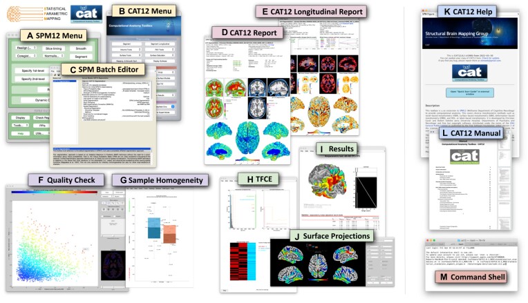
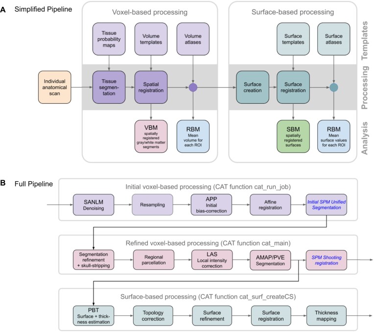
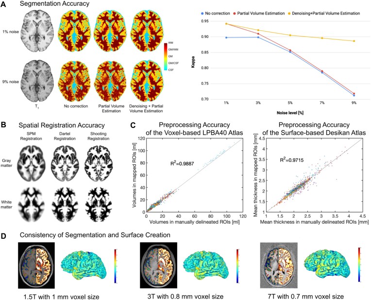
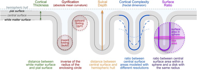
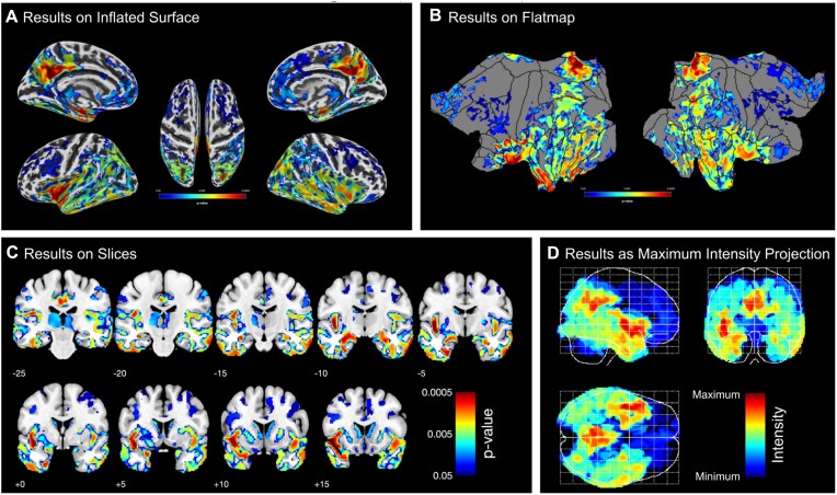
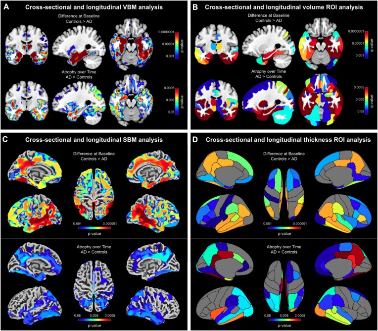
A large range of sophisticated brain image analysis tools have been developed by the neuroscience community, greatly advancing the field of human brain mapping. Here we introduce the Computational Anatomy Toolbox (CAT)-a powerful suite of tools for brain morphometric analyses with an intuitive graphical user interface but also usable as a shell script. CAT is suitable for beginners, casual users, experts, and developers alike, providing a comprehensive set of analysis options, workflows, and integrated pipelines. The available analysis streams-illustrated on an example dataset-allow for voxel-based, surface-based, and region-based morphometric analyses. Notably, CAT incorporates multiple quality control options and covers the entire analysis workflow, including the preprocessing of cross-sectional and longitudinal data, statistical analysis, and the visualization of results. The overarching aim of this article is to provide a complete description and evaluation of CAT while offering a citable standard for the neuroscience community.

Keywords: Alzheimer’s disease; CAT12; MRI; ROI; SPM12; VBM; brain; computational anatomy; cortical folding; cortical surface; cortical thickness; longitudinal; morphometry.

Figure 1:

Elements of the graphical user interface. The SPM menu (A) and CAT menu (B) allow access to the (C) SPM batch editor to control and combine a variety of functions. At the end of the processing stream, cross-sectional and longitudinal outputs are summarized in a brain-specific 1-page report (D, E). In addition, CAT provides options to check image quality (F) and sample homogeneity (G) to allow outliers to be removed before applying the final statistical analysis, including threshold-free cluster enhancement—TFCE (H); the numerical and graphical output can then be retrieved (I), including surface projections (J). For beginners, there is an interactive help (K) as well as a user manual (L). For experts, command line tools (M) are available under Linux and MacOS.

Figure 2:

Main processing streams. (A) Simplified pipeline: image processing in CAT can be separated into a mandatory voxel-based processing stream and an optional subsequent surface-based processing stream. Each stream requires different templates and atlases and, in addition, tissue probability maps for the voxel-based stream. The voxel-based stream consists of 2 main modules—for tissue segmentation and spatial registration—resulting in spatially registered (and modulated) gray matter/white matter segments, which provides the basis for voxel-based morphometry (VBM). The surface-based stream also consists of 2 main modules—for surface creation and registration—resulting in spatially registered surface maps, which provide the basis for surface-based morphometry (SBM). Both streams also include an optional module each to analyze regions of interest (ROIs) resulting in ROI-specific mean volumes (mean surface values, respectively). This provides the basis for region-based morphometry (RBM). (B) Detailed pipeline: to illustrate the differences from SPM, the CAT pipeline is detailed with its individual processing steps. The SPM methods used are shown in blue and italic font: images are first denoised by a spatially adaptive nonlocal means (SANLM) filter [15] and resampled to an isotropic voxel size. After applying an initial bias correction to facilitate the affine registration, SPM’s unified segmentation [16] is used for the skull stripping and as a starting estimate for the adaptive maximum a posteriori (AMAP) segmentation [17] with partial volume estimation (PVE) [18]. In addition, SPM’s segmentation is used to locally correct image intensities. Finally, the outcomes of the AMAP segmentation are registered to the MNI template using SPM’s shooting registration. The outcomes of the AMAP segmentation are also used to estimate cortical thickness and the central surface using a projection-based thickness (PBT) method [19]. More specifically, after repairing topology defects [20], central, pial, and white matter surface meshes are generated. The individual left and right central surfaces are then registered to the corresponding hemisphere of the FreeSurfer template using a 2D version of the DARTEL approach [21]. In the final step, the pial and white matter surfaces are used to refine the initial cortical thickness estimate using the FreeSurfer thickness metric [22, 23].

Figure 3:

Evaluation of segmentation and registration accuracy. (A) Segmentation Accuracy: Most approaches for brain segmentation assume that each voxel belongs to a particular tissue class, such as gray matter (GM), white matter (WM), or cerebrospinal fluid (CSF). However, the spatial resolution of brain images is limited, leading to so-called partial volume effects (PVE) in voxels containing a mixture of different tissue types, such as GM/WM and GM/CSF. As PVE approaches are highly susceptible to noise, we combined the PVE model [18] with a spatial adaptive nonlocal means denoising filter [15]. To validate our method, we used a ground-truth image from the BrainWeb [31] database with varying noise levels of 1–9%. The segmentation accuracy for all tissue types (GM, WM, CSF) was determined by calculating a kappa coefficient (a kappa coefficient of 1 means that there is perfect correspondence between the segmentation result and the ground truth). Left panel: The effect of the PVE model and the denoising filter on the tissue segmentation at the extremes of 1% and 9% noise. Right panel: The kappa coefficient over the range of different noise levels. Both panels demonstrate the advantage of combining the PVE model with a spatial adaptive nonlocal means denoising filter, with particularly strong benefits for noisy data. (B) Registration Accuracy: To ensure an appropriate overlap of corresponding anatomical regions across brains, high-dimensional nonlinear spatial registration is required. CAT uses a sophisticated shooting approach [24], together with an average template created from the IXI dataset [32]. The figure shows the improved accuracy (i.e., a more detailed average image) when spatially registering 555 brains using the so-called shooting registration and the Dartel registration compared to the SPM standard registration. (C) Preprocessing Accuracy: We validated the performance of region-based morphometry (RBM) in CAT by comparing measures derived from automatically extracted regions of interest (ROI) versus manually labeled ROIs. For the voxel-based analysis, we used 56 structures, manually labeled in 40 brains that provided the basis for the LPBA40 atlas [33]. The gray matter volumes from those manually labeled regions served as the ground truth against which the gray matter volumes calculated using CAT and the LPBA40 atlas were then compared. For the surface-based analysis, we used 34 structures that were manually labeled in 39 brains according to Desikan et al. [34]. The mean cortical thickness from those manually labeled regions served as the ground truth against which the mean cortical thickness calculated using CAT and the Desikan atlas were compared. The diagrams show excellent overlap between manually and automatically labeled regions in both voxel-based (left) and surface-based (right) analyses. (D) Consistency of Segmentation and Surface Creation: Data from the same brain were acquired on MRI scanners with different isotropic spatial resolutions and different field strengths: 1.5T MPRAGE with a 1-mm voxel size, 3T MPRAGE with a 0.8-mm voxel size, and 7T MP2RAGE with a 0.7-mm voxel size. Section Views: The left hemispheres depict the central (green), pial (blue), and white matter (red) surfaces; the right hemispheres show the gray matter segments. Rendered Views: The color bar encodes point-wise cortical thickness projected onto the left hemisphere central surface. Both section views and hemisphere renderings demonstrate the consistency of the outcomes of the segmentation and surface creation procedures across different spatial resolutions and field strengths.

Figure 4:

Cortical Measurements: Surface-based morphometry is applied to investigate cortical surface features (i.e., cortical thickness and various parameters of cortical folding) at thousands of surface points. Cortical Thickness: One of the best-known and most frequently used morphometric measures is cortical thickness, which captures the width of the gray matter ribbon as the distance between its inner boundary (white matter surface) and outer boundary (pial surface). Cortical Folding: CAT provides distinct cortical folding measures, derived from the geometry of the central surface: “Gyrification” is calculated via the absolute mean curvature [35] of the central surface. “Sulcal Depth” is calculated as the distance from the central surface to the enclosing hull [36]. “Cortical Complexity” is calculated using the fractal dimension of the central surface area from spherical harmonic reconstructions [37]. Finally, “Surface Ratio” is calculated as the ratio between the area of the central surface contained in a sphere of a defined size and that of a disk with the same radius [38].

Figure 5:

Examples of CAT’s visualization of results. Both surface- and voxel-based data can be presented on surfaces such as (A) the (inflated) FsAverage surface or (B) the flatmap of the Connectome Workbench. Volumetric maps can also be displayed as (C) slice overlays on the MNI average brain or (D) a maximum intensity projection (so-called glass brains). All panels show the corrected P values from the longitudinal VBM study in our example (see “Example application”).

Figure 6:

Pronounced atrophy in gray matter and cortical thickness in patients with Alzheimer’s disease compared to healthy control subjects. (A) Voxel-based morphometry (VBM) findings: Results were estimated using threshold-free cluster enhancement (TFCE), corrected for multiple comparisons by controlling the family-wise error (FWE), and thresholded at P < 0.001 for cross-sectional data and P < 0.05 for longitudinal data. Significant findings were projected onto orthogonal sections intersecting at (x = −27 mm, y = −10 mm, z = −19 mm) of the mean brain created from the entire study sample (n = 50). (B) Volumetric regions of interest (ROI) findings: ROIs were defined using the Neuromorphometrics atlas. Results were corrected for multiple comparisons by controlling the false discovery rate (FDR) and thresholded at q < 0.001 for cross-sectional data and q < 0.05 for longitudinal data. Significant findings were projected onto the same orthogonal sections as for the VBM findings. (C) Surface-based morphometry (SBM) findings: Results were estimated using TFCE, FWE-corrected, and thresholded at P < 0.001 for cross-sectional data and P < 0.05 for longitudinal data. Significant findings were projected onto the FreeSurfer FsAverage surface. (D) Surface ROI findings: ROIs were defined using the DK40 atlas. Results were FDR-corrected and thresholded at q < 0.001 for cross-sectional data and q < 0.05 for longitudinal data. Significant findings were projected onto the FsAverage surface.

References

1. SPM . https://www.fil.ion.ucl.ac.uk/spm. Accessed 1 July 2024.
1. FreeSurfer . https://surfer.nmr.mgh.harvard.edu. Accessed 1 July 2024.
1. Human Connectome Workbench . https://www.humanconnectome.org/software/connectome-workbench. Accessed 1 July 2024.
1. FSL . https://www.fmrib.ox.ac.uk/fsl. Accessed 1 July 2024.
1. BrainVISA . http://www.brainvisa.info. Accessed 1 July 2024.
MeSH terms
LinkOut - more resources