Revisiting Dominance in Population Genetics

Abstract

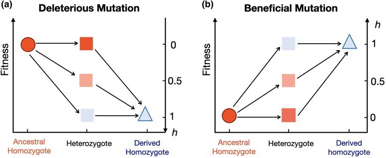
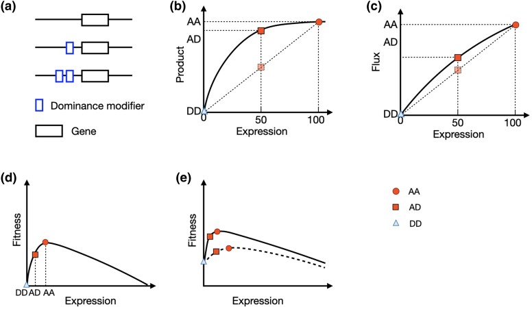
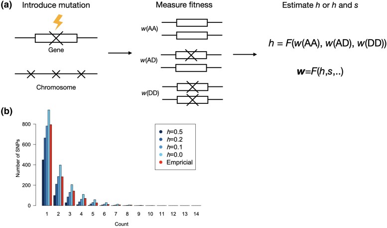
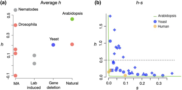
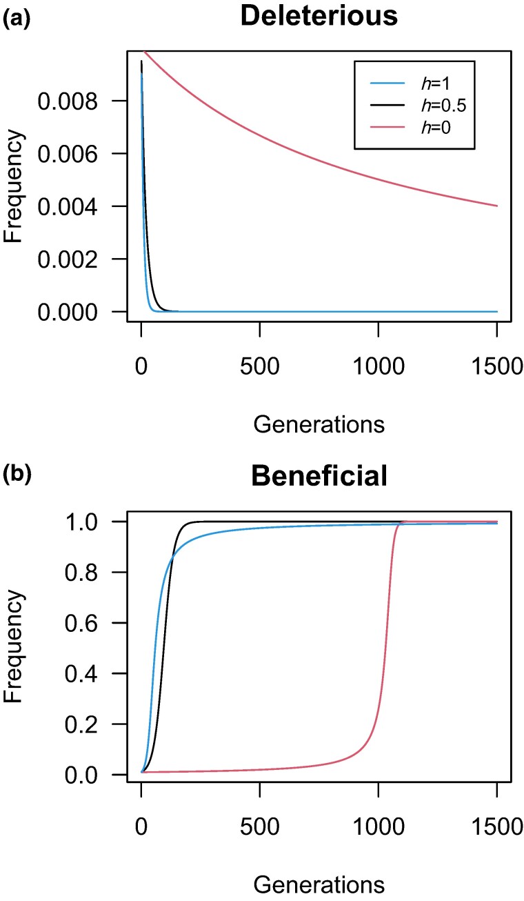
Dominance refers to the effect of a heterozygous genotype relative to that of the two homozygous genotypes. The degree of dominance of mutations for fitness can have a profound impact on how deleterious and beneficial mutations change in frequency over time as well as on the patterns of linked neutral genetic variation surrounding such selected alleles. Since dominance is such a fundamental concept, it has received immense attention throughout the history of population genetics. Early work from Fisher, Wright, and Haldane focused on understanding the conceptual basis for why dominance exists. More recent work has attempted to test these theories and conceptual models by estimating dominance effects of mutations. However, estimating dominance coefficients has been notoriously challenging and has only been done in a few species in a limited number of studies. In this review, we first describe some of the early theoretical and conceptual models for understanding the mechanisms for the existence of dominance. Second, we discuss several approaches used to estimate dominance coefficients and summarize estimates of dominance coefficients. We note trends that have been observed across species, types of mutations, and functional categories of genes. By comparing estimates of dominance coefficients for different types of genes, we test several hypotheses for the existence of dominance. Lastly, we discuss how dominance influences the dynamics of beneficial and deleterious mutations in populations and how the degree of dominance of deleterious mutations influences the impact of inbreeding on fitness.

Keywords: deleterious mutations; dominance; inference; natural selection; population genetics.

Fig. 1.

Dominance refers to the fitness of the heterozygous genotype compared with that of the homozygous genotypes. The left y-axis indicates the fitness of different genotypes (x-axis). a) For deleterious mutations, the ancestral homozygote (circle) has the highest fitness and the derived homozygote has the lowest fitness (triangle). The fitness of the ancestral homozygous genotype is 1, the derived (mutant) homozygote is 1−s, and the heterozygote is 1−hs. If the fitness of the heterozygote is the same as that of the ancestral homozygote (top square), h = 0 and the deleterious mutation is recessive. If the fitness of the heterozygote is the average of the ancestral and the derived homozygotes (middle square), h = ½, and the deleterious mutation is additive. If the fitness of the heterozygote is the same as the derived homozygote, h = 1, and the deleterious mutation is dominant (bottom square). b) For beneficial mutations, the ancestral homozygote has the lowest fitness (bottom left circle) and the derived homozygote has the highest fitness (upper right triangle). If the fitness of the heterozygote is the same as the ancestral homozygote (bottom circle), h = 0, the beneficial mutation is recessive (bottom square). If the fitness of the heterozygote is the average of the derived and ancestral homozygotes, the mutation is additive (middle square). If the fitness of the heterozygote is as high as that of the derived homozygote, the mutation is dominant and h = 1 (upper square).

Fig. 2.

Models explaining dominance. a) Fisher's dominance modifier model. Each line represents a small genomic region including a gene (black box). If there is no “dominance modifier” (the top line), a mutation in the gene is additive. Accumulation of the “dominance modifiers” increases the recessiveness of mutations. b) Wright's physiological model. Enzyme activity is shown on the x-axis. The y-axis indicates the enzyme-catalyzed reaction of different genotypes. The enzyme-catalyzed reaction can also be considered as an approximation to fitness in later models. The activity of the heterozygote (solid square) is very close to the fitness of the ancestral homozygote (circle) and much higher than the activity of the derived homozygote (triangle) because of the diminishing return. Adapted from fig. 6 of Kacser and Burns. c) Kacser and Burns' metabolic model. Similar to b) but in this example, there are fewer enzymes in the multiple-enzymes system. Consequently, here the flux of the heterozygote is close to the average of the ancestral and derived homozygotes. Adapted from fig. 4 of Kacser and Burns. d) Hurst and Randerson's optimal expression model. The y-axis indicates fitness and the x-axis indicates expression level, which is determined by the genotype. The ancestral homozygote has an optimal expression level (circle). Mutations decrease the expression level and fitness in the heterozygotes (square), and the expression and fitness drop to zero in the derived homozygote (triangle). Increasing gene expression beyond the optimal level decreases fitness due to the costs of increasing gene expression. e) Huber et al. (2018)'s modified optimal expression model is similar to d) but the fitness is above zero when the expression level of a non-essential gene is zero. The dashed line and solid line have different scale parameters reflecting different relationships between genotype and fitness. AA denotes genotypes homozygous for the ancestral allele, AD denotes heterozygous genotypes, and DD denotes genotypes homozygous for the derived allele.

Fig. 3.

Approaches to estimating dominance. a) Workflow of laboratory-based methods. The first step of experimental methods is to introduce mutations by deleting a gene, introducing mutations by chemical treatment, or allowing them to accumulate over time. Then, the fitness of heterozygotes, derived homozygotes, and ancestral homozygotes are either directly measured or approximated by some other measurements. Lastly, h and s are estimated from the fitnesses of the different genotypes using statistical models. b) The site frequency spectrum (SFS) is sensitive to the dominance of deleterious mutations. The SFS contains the number of variants (y-axis) at different frequencies in the sample (x-axis) from a population. Note, here we assume θ = 1,000 and 2Ns = −5. If deleterious mutations are more recessive, then they are more likely to segregate in the sample. To estimate h, the SFS from a hypothetical empirical sequencing dataset can be compared with that predicted by a model of dominance. Here the empirical SFS is closest to that from a model where h = 0.1. Note that the SFS was made using the theory presented in Williamson et al. (2004).

Fig. 4.

Estimates of dominance coefficients. a) Average h estimated by different methods. Dominance coefficients vary between species and across methods used for estimation. From left to right are estimates from mutations in mutation accumulation experiments (MA), mutations induced by EMS treatment, mutations from gene deletions, and mutations segregating in natural populations. Together, there are five estimates from Drosophila (red), three estimates from nematodes (gray), one from yeast (blue), and one from Arabidopsis (green). Estimates of the same group of mutations may differ because of the different statistical methods employed (see main text). b) Negative relationship between h and s. Each dot indicates an estimate of s and h. Mutations that are more deleterious (larger s) tend to be more recessive (smaller h). This trend is observed in yeast and humans, with different shapes indicating different studies of yeast. Note that the h−s relationship inferred by Huber et al. (2018) for Arabidopsis (solid line) is highly recessive. See supplementary table S1, Supplementary Material online for the raw data in this figure.

Fig. 5.

Dominance affects the dynamics of selected mutations in populations. a) Recessive deleterious mutations (h=0) decrease in frequency much more slowly due to selection than additive or dominant deleterious mutations. Here, s = 0.1. b) Beneficial mutations that are dominant (h=1) initially increase in frequency due to selection faster than additive or recessive beneficial mutations. Here, s = 0.1.

References

1. Abu-Awad D, Waller D. Conditions for maintaining and eroding pseudo-overdominance and its contribution to inbreeding depression. Peer Community J. 2023:3:e8. 10.24072/pcjournal.224. - DOI
1. Agrawal AF, Whitlock MC. Inferences about the distribution of dominance drawn from yeast gene knockout data. Genetics. 2011:187(2):553–566. 10.1534/genetics.110.124560. - DOI - PMC - PubMed
1. The Gene Ontology Consortium, Aleksander SA, Balhoff J, Carbon S, Cherry JM, Drabkin HJ, Ebert D, Feuermann M, Gaudet P, Harris NL, et al. The gene ontology knowledgebase in 2023. Genetics. 2023:224(1):iyad031. 10.1093/genetics/iyad031. - DOI - PMC - PubMed
1. Ashburner M, Ball CA, Blake JA, Botstein D, Butler H, Cherry JM, Davis AP, Dolinski K, Dwight SS, Eppig JT, et al. Gene ontology: tool for the unification of biology. Nat Genet. 2000:25(1):25–29. 10.1038/75556. - DOI - PMC - PubMed
1. Balick DJ, Do R, Cassa CA, Reich D, Sunyaev SR. Dominance of deleterious alleles controls the response to a population bottleneck. PLoS Genet. 2015:11(8):e1005436. 10.1371/journal.pgen.1005436. - DOI - PMC - PubMed
LinkOut - more resources