Encoding of 2D Self-Centered Plans and World-Centered Positions in the Rat Frontal Orienting Field

Abstract

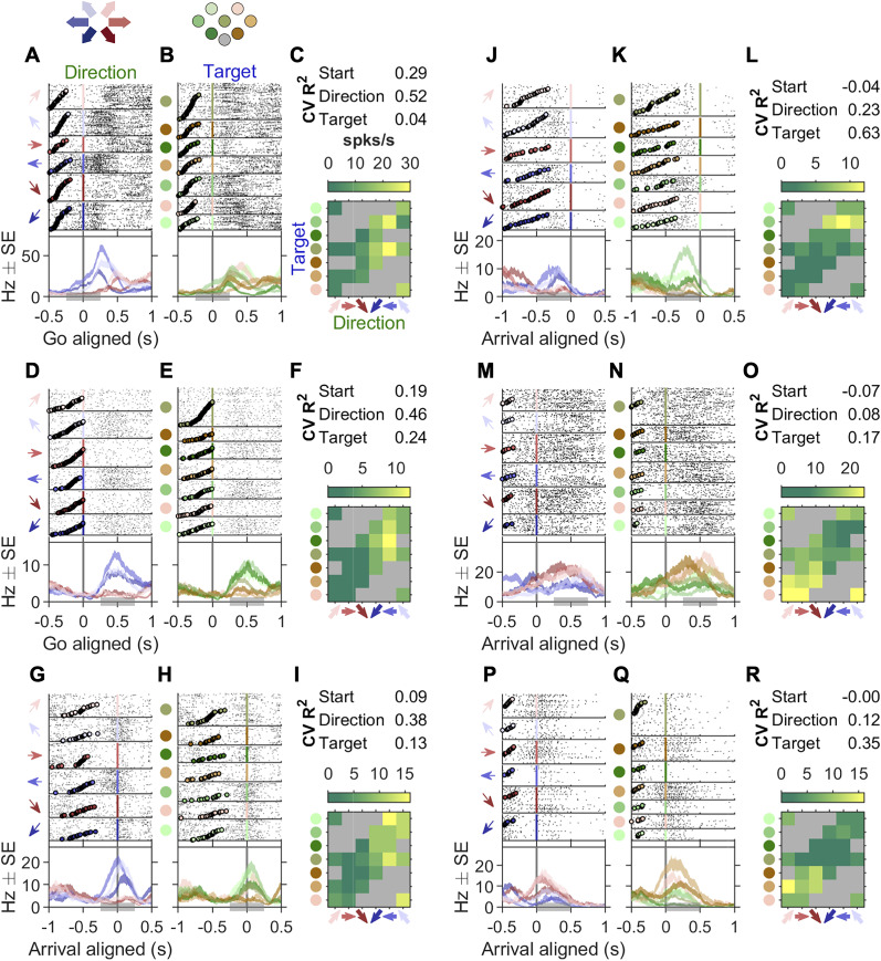
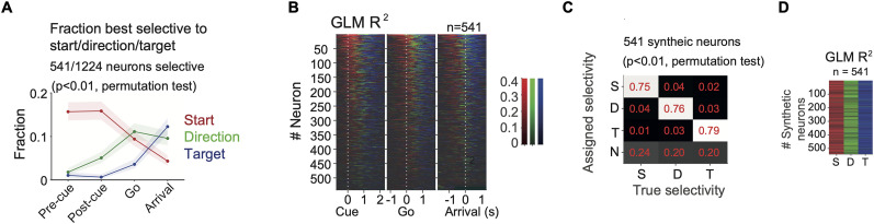
The neural mechanisms of motor planning have been extensively studied in rodents. Preparatory activity in the frontal cortex predicts upcoming choice, but limitations of typical tasks have made it challenging to determine whether the spatial information is in a self-centered direction reference frame or a world-centered position reference frame. Here, we trained male rats to make delayed visually guided orienting movements to six different directions, with four different target positions for each direction, which allowed us to disentangle direction versus position tuning in neural activity. We recorded single unit activity from the rat frontal orienting field (FOF) in the secondary motor cortex, a region involved in planning orienting movements. Population analyses revealed that the FOF encodes two separate 2D maps of space. First, a 2D map of the planned and ongoing movement in a self-centered direction reference frame. Second, a 2D map of the animal's current position on the port wall in a world-centered reference frame. Thus, preparatory activity in the FOF represents self-centered upcoming movement directions, but FOF neurons multiplex both self- and world-reference frame variables at the level of single neurons. Neural network model comparison supports the view that despite the presence of world-centered representations, the FOF receives the target information as self-centered input and generates self-centered planning signals.

Keywords: frontal cortex; motor planning; neural networks; neurophysiology; reference frame; rodent.

Figure 1.

A visually guided multi-directional orienting task in rats. A, Schematic of the task. Each trial began with the onset of a pair of blue and yellow LED, cuing the rat to nose poke into the start port. The start LED extinguished upon arrival in the start port. After a short delay, a blue LED illuminated, indicating the target port. After a go sound, the rat withdrew from the start port and poked into the target port. Water reward was delivered for correctly performed trials. B, Timeline of a trial in a typical session. Bars above the timelines illustrate the time windows used in the subsequent analyses. “Pre-cue,” −300 to 0 ms from visual cue onset. “Post-cue,” 0–300 ms from visual cue onset. “Go,” 0–300 ms from go sound. “Arrival,” −150 to 150 ms from target poke. C, The color scheme of the six movement directions. D, The color scheme of the seven port positions. E, The 30 movement trajectories consisted of 6 directions (shown in C). Each direction was associated with five possible trajectories, and there were four possible target ports associated with each direction. Each session only contained a subset of 16–24 trajectories among these trajectories, and these sessions were pooled together for analyses (see Methods for the details). F, The fraction of correct trials among all the completed trials. Dots and error bars denote mean ± s.e. across sessions. G, The proportion of errors made into the same left/right direction as instructed, among trials starting from the central port for each animal. Dots and error bars denote mean ± s.e. across sessions. H, The proportion of errors whose movement directions were lower, upper, or horizontal compared to the instructed movement direction. For each subject, the three dots and error bars denote the mean ± s.e. across sessions for the fraction of lower, upper, and horizontal errors. For subject 2095 and 2134, there were significantly more downward errors than upward errors. I, The range of fixation periods experienced by each rat, shown as a cumulative distribution. The color of the lines correspond to the colors of the labels in F. J, Example traces of the horizontal head position in the video pixel space during trials starting from the central port. The traces were aligned to the visual cue onset. Each line is a trial, and the colors indicate the movement directions. K, There was no significant correlation between the horizontal head position and the planned movement direction before the go cue. The line indicates p-value of the movement direction modulation on the horizontal head position across time aligned to the go sound. All the correctly performed trials were included and the effect of start position was captured in the random effect. Line and error bars, mean ± s.d. of the p-values over the 58 sessions.

Figure 2.

Schematics of the task and histology. A, Three trajectories that can distinguish between tuning to the start position, movement direction, or the target position (left) and the predicted neural activities for each scenario. Among the three trials, the orange and pink trials share the start position, the blue and pink trials share the movement direction, and the blue and orange trials share the target position. If a neuron is tuned to the start position, then the firing rate in the pink and orange trials will be the same, but not for the blue trial. The same logic follows for direction tuning and target tuning cells. B, A coronal section from an example rat (2147) showing the placements of the silicon probes. Dashed lines indicate the estimated area of M2 in this brain section. C, Estimated positions of the tips of the silicon probes at the end of recording presented on coronal sections of the rat brain atlas (Paxinos and Watson, 2004). Lesions were made at the end of all the recording sessions with 200 uA current for 3 s relative to the ground. Colored marks indicate the lesion marks in B, and colors indicate subject ID.

Figure 3.

Example neurons with egocentric and allocentric spatial representation. A–C, An example neuron more modulated by the egocentric movement directions than by the allocentric target positions. A, Raster plots and PETHs aligned to the go sound and sorted by movement directions. The top six panels show spike rasters grouped by the six movement directions. Circles in each raster panel indicate the time of the visual cue onset on each trial. The bottom panel shows the PETHs of the spikes. The shaded areas of the PETHs indicate the mean ± s.e. The gray bar at the bottom of the panel indicates the 500 ms time window used to estimate the cross-validated R²s and the firing rate for each movement trajectory in C. B, Raster plots and PETHs of the same cell and same alignment as in A, but sorted by target position. Circles in each raster panel indicate the time of visual cue onset on each trial. C, CV R². The cross-validated R²s of three GLMs whose independent variables were the start position, movement direction or target position (See Methods for definition). Heat map. The maximum a posteriori estimated firing rate for each movement trajectory, where the prior was a Poisson distribution whose mean was estimated from all trials. Gray squares indicate trajectories (direction-target pairs) that were not included in that session. D–F and G–I, two more example cells as in A–C where direction explained the most variance than start or target positions. Note that in G,H the activity is aligned to arrival. J–L, M–N, and P–R, example neurons whose arrival-aligned activity was more modulated by the target position than direction. Circles in each raster panel indicated the time of the go sound.

Figure 4.

Temporal profile of the fraction of FOF neurons best selective to the start position, direction, and target position. A, The fraction of neurons best selective to the start position (red), the direction, (green) or the target position (blue) in four time windows. Shaded areas indicate the 95% binomial confidence intervals. “Pre-cue,” −300 to 0 ms to visual cue onset. “Post-cue,” 0–300 ms to visual cue onset. “Go,” 0 to 300 ms to go sound. “Arrival,” −150 to 150 ms to target poke as in Figure 1B. B, The R² of GLMs among same neurons as in A in 300 ms causal sliding windows with 50 ms steps, aligned to the cue onset, go sound or target arrival. At each time point, the color represents the variable with the largest R² and the saturation represents the R² value. Neurons were sorted by the total mass of the R²s of start position, direction and target position for the three alignments respectively. C, Fraction of synthetic neurons most selective to each generative spatial variable. Each column represents 541 synthetic neurons that were designed to be selective to start position (S), direction (D), or target position (T), or nonselective (N). The vast majority of errors were false negatives (where a neuron was incorrectly labeled nonselective). D, The R²s of GLMs in synthetic neurons with specific spatial selectivity. Each column was a group of 541 synthetic neurons selective to start, direction or target, respectively. The color indicated the R² of the model with the maximum R², with the same scale as in B.

Figure 5.

The sequential encoding of start position, direction, and target position was consistent across single-neuron selection criteria and across subjects. A, The fraction of units with significant spatial selectivity at different cut-off criteria for the in-trial firing rate. The cutoff of the signal-to-noise ratio (SNR) of the waveform was fixed at 5. A unit is characterized as having significant spatial selectivity if any one of the three GLMs had p < 0.01 (permutation test) for any one of the four time windows (“pre-cue,” “post-cue,” “go,” or “arrival”). B, The fraction of units with significant spatial selectivity at different cut-off criteria for the SNR of the waveform. The cut-off criteria for in-trial firing rate was fixed at 1 Hz. C, The number of units with significant spatial selectivity at different in-trial firing rate cutoff. D, The number of units with significant spatial selectivity at different SNR cutoffs. E, Similar to Figure 4A, but the cut-off criteria is SNR >6 and in-trial firing rate >2 Hz instead of SNR >5 and firing rate >1 Hz. F, Similar to Figure 4A, but for each subject.

Figure 6.

Temporal profile of start position, direction, and target position decoding from the FOF pseudopopulation. A, Number of principle components included versus the accuracy of pseudopopulation decoding for the start position, using spike count data in the pre-cue time window. Thin line and shaded areas indicated the mean and the 5% and 95% intervals in 100 pseudopopulations with neurons resampled with replacement. Error is defined as the Euclidean distance between the predicted and the actual coordinates. B, Decoded coordinates of start position, movement vector, and target position in an example pseudopopulation. Each small circle indicates the predicted coordinates in a pseudo-trial, and the color indicates the pseudo trial class. Each large circle indicates the coordinates and the radius of a port (11 mm). C, Decoding errors for each pseudopopulation across time aligned to the go sound. Each row is a different pseudopopulation, and the color indicates decoding error following the color bar in E. Red solid lines indicate the mean errors across the 100 pseudopopulations. Red dashed lines indicate the radius of the ports. D, Mean ± s.d. of the difference of decoding errors between two spatial variables across the 100 pseudopopulations. Positive difference indicates the better decoding of the second variable, and vice versa. E, Decoding errors with cross-window decoding. Colors of the heat maps indicate the mean Euclidean distance between the decoded and true spatial coordinates, averaged across 100 pseudopopulations. The decoders were trained at one time window and tested at another. In the last panel, the multivariate linear model was trained for start position and decoded for target position. Contours, p < 0.01 (extreme pixel-based test). Pseudopopulations were constructed from neurons with at least eight trials for each of the six directions, seven start positions and seven target positions (n = 1, 197).

Figure 7.

FOF neurons were tuned to specific positions. A, Raster plots and PETHs of an example neuron aligned to the cue, grouped by start position. The shaded gray area indicates the time window to calculate the x-axis firing rate in C. The neuron was the same one as in Figure 3P–R. B, the same neuron aligned to target arrival, grouped by target position. C, The correlation between start position tuning and target position tuning in the example neuron. Red line denotes the total least-square fit. r denotes the Pearson correlation between start and target tuning, which was termed start-target tuning correlation. D, The distribution of the start-target tuning correlation among start and (or) target selective neurons. Black bars are for neurons selective to both start position and target position, and white bars are for neurons selective to only one of the two variables (mean, [95% CI]: 0.66, [0.61, 0.70] for both selective and 0.29, [0.25, 0.34] for only 1 selective). Triangles indicate the means of the two groups. E, The start-target tuning correlation in warped time windows aligned to the visual cue, the go sound and the arrival, averaged across neurons with both start and target selectivity (n = 174). The white contours indicate the areas where correlation is significantly larger than 0 (p < 0.05 after Bonferroni correction). Different from C and D, these correlations were calculated between start tuning in half of the trials and target tuning in the other half of trials and vice versa, and then averaged. F, Similar to E, but for the mean Pearson correlation between pairs of time windows for start position tuning in one half of trials versus the start tuning in the other half. G, Similar to F, but for target position tuning. H, Time of transition from start position coding to target position coding in the 174 neurons. The color of the heat map indicates the difference between R²s of the start position GLM and the target position GLM, calculated at causal sliding 300 ms time windows of 50 ms step size aligned to the go sound. The red dots indicate the time of switching from $R_{\mathrm{start}}^2$ higher to $R_{target}^2$ higher. The white crosses indicate the averaged time of target poke for that session. I, The number of neurons preferring each start position in the “pre-cue” time window, among cells that had significant start position selectivity in the “pre-cue” window (p < 0.01, permutation test for the start position GLM). J, The number of cells preferring each target position in the “arrival” time window, among cells that have significant target position selectivity in that window (p < 0.01, permutation test for the target position GLM).

Figure 8.

Direction preference of FOF neurons. A, The distribution of preferred direction in the “go” time window (0–300 ms after the go sound) among 274 cells that had significant direction selectivity in either the “post-cue” or “go” time windows (p < 0.01, permutation test for the GLM). Note, that the color scheme here represents ipsilateral versus contralateral to the recording side in the horizontal direction (as opposed to right vs left in other figures). B, The preferred direction of neurons in A in causal sliding windows aligned to the go sound (50 ms step size, 300 ms bin size). The color indicates the preferred angle (as in A) and the saturation indicates the relative amplitude of the R² of the direction GLM. The neurons were sorted by the preferred direction in the “go” time window. The color map on the right demonstrates the full saturation color for that preferred direction in the “go” time window. R² = 0.69 was the largest R² for the direction GLM, and was used to define the full saturation color. C, Pearson correlation of direction tuning curves at one time versus another, among the 274 neurons in A and B. Colors indicate the mean correlation across these neurons. White contour indicates the area with where correlation was significantly larger than zero with Bonferroni correction (p < 0.05).

Figure 9.

The spatial selectivity of FOF neurons were best explained by the gain-field model. A, Raster plots and PETHs of an example neuron. Trials were grouped by the start position (left panel), the direction (middle panel), and the target position (right panel). The gray bar at the bottom indicates the 500 ms time window after the visual cue onset, the time window used for firing rate estimation, and model fitting in B–E. B, Estimated mean firing rate in each movement trajectory using a maximum a posterior estimator, same as in Figure 3. C, Predicted firing rates of four fit models (lines) and the mean and s.e. (circles and error bars) of firing rates in each trial condition. CV R², cross-validated R² (see Methods for definition). D, Left axis, fraction of neurons best fit by a specific model, among neurons whose mean cross-validated R²s over the four models was larger than the x-axis indicated value. Best fit was defined as having the largest cross-validated R² among the four models. Error bars were 95% confidence intervals of the binomial distribution. Right axis, neurons that crossed the mean CV R² criteria for each x-axis value. E, Each panel plots the cross-validated R²s of the x-axis model versus the y-axis model. Each circle indicates a neuron. The red line indicates the total least-square fit to the data. The dashed black line marks the diagonal. Only neurons whose mean of cross-validated R²s in the four models were larger than 0.05 were included (n = 199). The mean R² in the gain-field model was larger than the x-axis models in all of these panels. ***, p < 0.001 (gain field vs additive, p = 8 × 10⁻⁵; gain field vs direction, p = 2 × 10⁻⁵; gain field vs start, p = 2 × 10⁻⁵. Permutation test against the null hypothesis that the Fisher-z transformed cross-validated R²s in the x-axis model and the y-axis model was not significantly different from zero, with 10⁵ shuffles). F, The cross-validated R²s of the additive model versus the gain-field model in synthetic neurons, designed to have additive or gain-field selectivity, respectively. Only synthetic neurons whose cross-validated R²s in the four models were larger than 0.05 were included. Both panels had p = 2 × 10⁻⁵ (permutation test same as in E).

Figure 10.

Design of RNN simulations with four types of input–output contingencies. A, The schematics of the models. The input to the RNN was a figure that was down-sampled and flattened. The elements in the figure was intensity-coded and pseudo-colored for demonstration purpose. The output was a two-element vector of the x and y coordinates. B, The timeline of a trial and the input–output contingency for an example world frame. The trial consists of 11 time frames, where the target port was transiently visible on the 4th frame. In ego-input models, the start position was always at the center of the visual frame, whereas in allo-input models, the world frame was always at the center of the visual frame. On time frame 11, allo-output models were required to output the target position and ego-output models were required to output the movement vector. The time frames 3, 7, and 11 were designated as the pre-cue, post-cue, and go windows to compare with data from FOF neurons.

Figure 11.

FOF population activity was most similar to a recurrent network with self-centered input and self-centered output. A, Left, same as Figure 4A. Right, the cross-validated R²s from a linear model that decodes the start position, movement vector, or target position from hidden unit activities. Shaded area denoted the standard error of the mean over 20 training and testing epochs. The ego-ego network had the most similar temporal pattern of decoding accuracy as the FOF neurons. B, The representational similarity between the FOF neural population activity and the population activity in RNNs, computed with the first four principle components of pseudopopulation activity in the FOF neural data and the network hidden unit data. Colors denote the representation similarity averaged across 20 RNN training epochs. C, The representation similarity between the FOF neural population activity and the network hidden unit activity at the diagonal of B. Circles and error bars were mean and s.d. from 20 training and testing epochs. Representation similarity of the ego-ego models were significantly higher than other models in post-cue and go windows (Table 3). D, Example units in the four networks that had gain-field-like selectivity to start position and direction. Each dot is a trial and each line is the average over trials with the same start position which is indicated by color.

References

1. Alexander AS, Robinson JC, Stern CE, Hasselmo ME (2023) Gated transformations from egocentric to allocentric reference frames involving retrosplenial cortex, entorhinal cortex, and hippocampus. Hippocampus 33:465–487. 10.1002/hipo.23513 - DOI - PMC - PubMed
1. Andersen R, Bracewell R, Barash S, Gnadt J, Fogassi L (1990) Eye position effects on visual, memory, and saccade-related activity in areas LIP and 7a of macaque. J Neurosci 10:1176–1196. 10.1523/JNEUROSCI.10-04-01176.1990 - DOI - PMC - PubMed
1. Andersen R, Essick G, Siegel R (1985) Encoding of spatial location by posterior parietal neurons. Science 230:456–458. 10.1126/science.4048942 - DOI - PubMed
1. Andersen R, Mountcastle V (1983) The influence of the angle of gaze upon the excitability of the light-sensitive neurons of the posterior parietal cortex. J Neurosci 3:532–548. 10.1523/JNEUROSCI.03-03-00532.1983 - DOI - PMC - PubMed
1. Bao C, Zhu X, Li J, Dubroqua S, Erlich JC (2023) The rat frontal orienting field dynamically encodes value for economic decisions under risk. Nat Neurosci 26:1942–1952. 10.1038/s41593-023-01461-x - DOI - PMC - PubMed
LinkOut - more resources