Causal evidence of a line attractor encoding an affective state

Abstract

Continuous attractors are an emergent property of neural population dynamics that have been hypothesized to encode continuous variables such as head direction and eye position^1-4. In mammals, direct evidence of neural implementation of a continuous attractor has been hindered by the challenge of targeting perturbations to specific neurons within contributing ensembles^2,3. Dynamical systems modelling has revealed that neurons in the hypothalamus exhibit approximate line-attractor dynamics in male mice during aggressive encounters⁵. We have previously hypothesized that these dynamics may encode the variable intensity and persistence of an aggressive internal state. Here we report that these neurons also showed line-attractor dynamics in head-fixed mice observing aggression⁶. This allowed us to identify and manipulate line-attractor-contributing neurons using two-photon calcium imaging and holographic optogenetic perturbations. On-manifold perturbations yielded integration of optogenetic stimulation pulses and persistent activity that drove the system along the line attractor, while transient off-manifold perturbations were followed by rapid relaxation back into the attractor. Furthermore, single-cell stimulation and imaging revealed selective functional connectivity among attractor-contributing neurons. Notably, individual differences among mice in line-attractor stability were correlated with the degree of functional connectivity among attractor-contributing neurons. Mechanistic recurrent neural network modelling indicated that dense subnetwork connectivity and slow neurotransmission⁷ best recapitulate our empirical findings. Our work bridges circuit and manifold levels³, providing causal evidence of continuous attractor dynamics encoding an affective internal state in the mammalian hypothalamus.

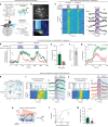
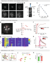
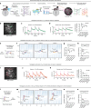
Fig. 1. Attractor dynamics in head-fixed mice observing aggression.

a, The experimental paradigm for 2P imaging in head-fixed mice observing aggression. b, Representative FOV through a GRIN lens in the 2P set-up (top). Bottom, fluorescence image of a coronal slice showing expression of jGCaMP7s and ChRmine. Scale bars, 100 µm. c, Neural and behavioural raster from an example mouse observing aggression in the 2P set-up (left). The arrows indicate insertion of submissive BALB/c intruders into the observation chamber for interaction with an aggressive Swiss Webster (SW) mouse. Right, example neurons from the raster to the left. d, Neural activity projected onto rSLDS dimensions obtained from models fit to 2P imaging data in one example mouse. e, rSLDS time constants across mice. n = 9 mice. Statistical analysis was performed using two-tailed Mann–Whitney U-tests. Data are mean ± s.e.m. f, The line-attractor score (Methods) across mice. n = 9 mice. Data are mean ± s.e.m. g, Behaviour-triggered average of x₁ and x₂ dimensions, aligned to the introduction of BALB/c mice into the resident’s cage. n = 9 mice. Data are the average activity (dark line) ± s.e.m. (shading). h, Flow fields from rSLDS model fit to 2P imaging data during observation of aggression from one example mouse. The larger blue arrows next to the neural trajectory indicate the direction flow of time. The smaller arrows represent the vector field from the rSLDS model. i, Identification of neurons contributing to x₁ dimension from rSLDS model (top). The neuron’s weight is shown as an absolute (abs) value. Bottom, activity heat map of five neurons contributing most strongly to the x₁ dimension. Right, neural traces of the same neurons and an indication of when the system enters the line attractor. j, As in i but for the x₂ dimension. k, Dynamic velocity landscape from 2P imaging data during observation of aggression from one example mouse. Blue, stable area in the landscape; red, unstable area in the landscape. The black line shows the trajectory of neuronal activity. l, The cumulative distributions of the autocorrelation half width (ACHW) of neurons contributing to the x₁ (green) and x₂ (red) dimensions. n = 9 mice, 45 neurons each for the x₁ and x₂ distributions. m, The mean autocorrelation half width (HW) across mice for neurons contributing to the x₁ and x₂ dimensions. n = 9 mice. Statistical analysis was performed using a two-tailed Mann–Whitney U-test; **P = 0.0078. Data are mean ± s.e.m. ****P < 0.0001, **P < 0.01.

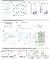
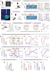
Fig. 2. Holographic perturbations reveal integration dynamics in the VMHvl.

a, The experimental paradigm for 2P perturbation in head-fixed mice. b, FOV of five x₁ neurons selected for 2P activation in example mouse 1. Scale bar, 100 µm. c, Neural activity projected onto the x₁ dimension after holographic activation of five x₁ neurons in example mouse 1. The pink vertical lines show the time of activation. d, The average activity projected onto the x₁ dimension from activation of 5 x₁ neurons (left). Data are average (dark green) ± s.e.m. (shaded green area). n = 8 mice. Right, the average z-scored activity of the projected x₁ dimension during the baseline or ISIs. n = 8 mice. Statistical analysis was performed using Kruskal–Wallis tests with Dunn’s correction; *P = 0.0363, **P = 0.0013 (bottom), **P = 0.0067 (top). Data are mean ± s.e.m. e, Schematic of quantifying perturbation along line attractor in neural state space. f, Flow fields from example mouse 1, showing perturbations along the line attractor after activation of 5 x₁ neurons. The larger blue arrows next to the neural trajectory indicate the direction flow of time. The smaller arrows indicate the vector field from the rSLDS model. g, The Euclidian distance between time points t_initial and t_stim-end across mice. n = 8 mice. Statistical analysis was performed using Kruskal–Wallis tests with Dunn’s correction; not significant (NS), P = 0.061; *P = 0.029, **P = 0.0018 (bottom), **P = 0.0059 (top). Data are mean ± s.e.m. h, As in g but for timepoints t_initial and t_post-stim. n = 8 mice. Statistical analysis was performed using Kruskal–Wallis tests with Dunn’s correction; NS, P = 0.1965; **P = 0.0082, ***P = 0.0004, *P = 0.016. Data are mean ± s.e.m. i, FOV of five x₂ neurons selected for activation in example mouse 1. Scale bar, 100 µm. j, Neural activity projected onto the x₂ dimension after holographic activation of x₂ neurons in example mouse 1. k, The average activity projected onto the x₂ dimension from activation of x₂ neurons (left). Data are average (dark red) ± s.e.m. (shaded red area). n = 7 mice. Right, the average z-scored activity of the projected x₂ dimension during the baseline or ISIs. n = 7 mice. Statistical analysis was performed using Kruskal–Wallis tests with Dunn’s correction; P > 0.99. Data are mean ± s.e.m. l, As in e but for x₂ activation. m, Flow fields from example mouse 1, showing x₂ activation. The red arrows indicate the direction of the flow of time. n, As in g but for x₂ activation. n = 7 mice. Statistical analysis was performed using Kruskal–Wallis tests with Dunn’s correction; NS, P = 0.1554; *P = 0.042 (bottom), *P = 0.029 (middle), *P = 0.029 (top). Data are mean ± s.e.m. o, As in h but for x₂ activation. n = 7 mice. Statistical analysis was performed using Kruskal–Wallis tests with Dunn’s correction; NS, P > 0.05 (bottom), P = 0.508 (middle), P = 0.0508 (top); *P = 0.0383. Data are mean ± s.e.m. NS, P > 0.05; *P < 0.05, ***P < 0.001, ****P < 0.0001.

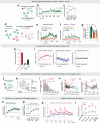
Fig. 3. Neural implementation of a line attractor by functional connectivity.

a, Left, the paradigm for examining activity in non-targeted x₁ and x₂ neurons after activation of unitary x₁ neurons. Right, the average z-scored activity of the perturbed (targeted) x₁ neurons (25 single neurons from n = 8 mice). Data are the average trace (dark green) ± s.e.m. (shaded green area). b, The average z-scored activity of non-targeted x₁ neurons after targeting unitary x₁ neurons. n = 8 mice. Data are average trace (dark green) ± s.e.m. (shaded green area). c, The average z-scored activity of non-targeted x₂ neurons after targeting of unitary x₁ neurons. n = 8 mice. Data are average (trace in dark red) ± s.e.m. (shaded red area). d, Quantification of activity in non-targeted x₁ neurons after targeting of single x₁ neurons. NS, P = 0.16; **P = 0.0037 (bottom), ***P = 0.0005, **P = 0.0016 (top). n = 8 mice. Data are mean ± s.e.m. e, Quantification of the activity in non-targeted x₂ neurons after targeting of single x₁ neurons (NS; n = 8 mice). Data are mean ± s.e.m. f, The paradigm for examining the activity in non-targeted x₁ and x₂ neurons after activation of single x₂ neurons (left). Right, the average z-scored activity of targeted x₂ neurons (18 single neurons from n = 7 mice). Data are the average trace (dark red) ± s.e.m. (shaded red area). g, The average z-scored activity of non-targeted x₂ neurons after targeting of single x₂ neurons. n = 7 mice. Data are the average trace (dark red) ± s.e.m. (shaded red area). h, The average z-scored activity of non-targeted x₁ neurons after targeting of single x₂ neurons. n = 7 mice. Data are the average trace (dark green) ± s.e.m. (shaded green area). i, Quantification of activity in non-targeted x₁ neurons after targeting of single x₂ neurons. NS, from bottom to top, P = 0.999, P = 0.31, P = 0.09; *P = 0.0316. n = 7 mice. Data are mean ± s.e.m. j, Quantification of activity in non-targeted x₂ neurons after targeting of single x₂ neurons (NS). n = 7 mice. Data are mean ± s.e.m.

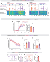
Fig. 4. Mechanistic modelling suggests slow neurotransmission and feedback inhibition.

a, Diagram of strong but sparse connectivity among x₁ neurons (1), or dense interconnectivity within subnetwork (2) (left). Right, the empirical distribution of the strength of pairwise functional connectivity between x₁ neurons (green) and from x₁ to x₂ neurons (red). n = 99 pairs, n = 7 mice. b, Cartoon illustrating different elements of an excitatory network that can determine network-level persistent activity. c, Model simulation result showing the network time constant (τ_n) by varying the subnetwork connectivity (σ) in the range of 0 to 20% density values and τ_s in the range of 0 to 20 s. Blue portions show configurations that result in unstable networks with runaway excitation. d, Magnified version of c (the region left of the dashed line) showing glutamatergic networks with a synaptic conductance time constant (τ_s) in range of 0.01 to 0.6 s. e, Network time constant (τ_n) against density of integration subnetwork for slow neurotransmitter (τ_s: 10, 15 and 20 s). τ_n varies monotonically with density for large values of τ_s. f, As in e but for glutamatergic networks (τ_s: 0.01, 0.1, 0.2 and 0.3 s). g, Cartoon showing the modified VMHvl circuit with fast feedback inhibition incorporated. h, Plot of network time constant (τ_n) against density of integration subnetwork for a slow neurotransmitter network with τ_s = 20s, for different values of strength of inhibition (inhibitory gain, g_inh: 1.25, 5 and 10) (left). Right, as on the left but for a glutamatergic network with t_s = 0.1 s. i, Model simulation of a slow neurotransmitter network with fast feedback inhibition (t_s: 20 s, 36% density of subnetwork connectivity). Top, the input (20 s ISI) provided to the model, Bottom, spiking activity in the network. The first 200 neurons (20%) comprise the interconnected integration subnetwork. j, Ca²⁺ activity convolved from firing rate (Methods) of the integration subnetwork (top) and the remaining neurons (bottom). k, As in i but for a fast transmitter network (t_s: 0.1 s, 36% density of subnetwork connectivity). l, As in j but for a fast transmitter network (t_s: 0.1 s, 36% density of subnetwork connectivity). a.u., arbitrary units.

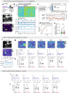
Fig. 5. The strength of functional connectivity reflects line-attractor stability.

a, Example neural activity projected onto the x₁ (integration) dimension (dimen.) of one mouse observing aggression, demonstrating a ramp when the BALB/c intruder enters the demonstrator cage containing an aggressive SW mouse (that is, movement up the line attractor) and decay after removal of the BALB/c intruder from the demonstrator cage (that is, movement down the line attractor). b, Dynamics of the integration dimension aligned to the entry of the BALB/c intruder for three example mice. Note the different rates of ramping in different mice. Norm. act., normalized activity. c, As in b, aligned to the removal of the BALB/c intruder, showing different rates of decay. d, z-scored activity of non-targeted x₁ neurons after activation of individual x₁ neurons in mice from b and c. The pink vertical lines show photostimulation pulses. e, Illustration of different quantitative metrics of the change in activity of non-targeted x₁ neurons from d as either the average z-scored activity, or the area under the curve (AUC). The pink vertical lines show the photostimulation pulses. f, Correlation between the rate of ramping of the integration dimension from the rSLDS model fit to data obtained from observation of aggression, and the AUC of non-targeted x₁ neurons measured using AUC after the third stimulus (r² = 0.01; NS). n = 8 mice. g, The correlation between the rSLDS time constant (decay rate of the integration dimension) obtained from observation of aggression, and the AUC of non-targeted x₁ neurons measured after the third stimulus (R² = 0.87; ***P < 0.001). n = 8 mice. h, Summary of the results illustrating causal evidence of a hypothalamic line attractor. i, Diagram of the implementation of a hypothalamic line attractor encoding a behavioural internal state.

Extended Data Fig. 1. Shared line attractor dynamics in freely behaving mice engaging in or observing aggression.

a. Implantation of miniscope, field of view (top) and fluorescence image showing histology (bottom) with jGCaMP7s expression in VMHvl. N = 5 mice. b. Experimental paradigm to record VMHvl^Esr1 activity in mice engaging in aggression. c. Left: neural & behavioural raster of example mouse 1 when engaging in aggression. Right: example neurons. d. Experimental paradigm to record VMHvl^Esr1 activity in same mice in Extended Data Fig. 1c during observation of aggression. e. Left: neural & behavioural raster of example mouse 1 during observation of aggression. Right: example neurons. f. Overview of rSLDS analysis. g. Left: rSLDS time constants in example mouse 1. Right: Normalized neural activity projected onto two dimensions (x₁ and x₂) of dynamical system. h. Behaviour triggered average of normalized x₁ and x₂ dimensions, aligned to introduction of male intruder (n = 5 mice, average trace in dark red and black ± sem in shaded area). i. Behaviour triggered average of x₁ dimensions, aligned to first attack onset (n = 5 mice, average trace in dark red ± sem in shaded red area). j. Left: rSLDS time constants in example mouse 1 during observation of aggression. Right: Neural activity projected onto two dimensions (x₁ and x₂) of dynamical system. k. Behaviour triggered average of normalized x₁ and x₂ dimensions from observation of aggression, aligned to introduction of BALB/c into resident’s cage (n = 5 mice, average trace in dark purple and black ± sem in shaded area). l. Behaviour triggered average of x₁ dimensions from observation of aggression, aligned to first bout of observing attack (n = 5 mice, average trace in dark purple ± sem in shaded purple area). m. Average activity in the x₁ dimension during sniffing of the SW mouse, vs observing the SW mouse a BALB\c intruder (n = 4 mice, *p = 0.0286, Two-tailed Mann Whitney U-test, error bars - sem). n. rSLDS time constants across mice engaging in aggression (n = 5 mice, *p = 0.0079, Two-tailed Mann Whitney U-test, error bars - sem). o. Line attractor score across mice engaging in aggression (n = 5 mice, error bars - sem). p. rSLDS time constants across mice during observation of aggression (n = 5 mice, *p = 0.0079,Two-tailed Mann Whitney U-test, error bars - sem). q. Line attractor score across mice during observation of aggression (n = 5 mice, error bars - sem).

Extended Data Fig. 2. Flow fields from miniscope experiments during engagement and observation of aggression.

Flow fields from all mice showing neural trajectories aligned to removal of the intruder or demonstrator mouse in either observation or engagement of aggression. Dashed lines highlight region of slow points (line attractor).

Extended Data Fig. 3. Comparing neuronal activity of x₁ neurons during engaging vs. observing aggression.

a. Normalized neuronal activity of all x₁ neurons from example mouse 1 when engaging in aggression (left) and observing aggression (right). Bottom: Raster plots of the activity of all neurons from x₁ dimension in mouse 1. b. Same as in panel a but for example mouse 2. c. comparing the activity of x₁ neurons between observing and engaging in aggression. Left: Average activity across mice (n = 5 mice, shaded area is sem). Right: comparison of the activity during observing attack bouts and engaging in attack (n = 5 mice, p = 0.42, Two-tailed Mann-Whitney U-test, error bars - sem). d. Activity of x₁ neurons aligned to removal of last intruder during observation and engaging in aggression (n = 5 mice, shaded area is sem). e. Quantification of autocorrelation half-width for x₁ neurons in both conditions during the full interaction (mean achw during observation: 25 ± 0.8s, mean achw during engagement: 20 ± 1.7s, n=5 mice, p = 0.125, Two-tailed Mann-Whitney U-test, error bars - sem). f. Quantification of achw for x₁ neurons in both conditions aligned to removal of last intruder (mean achw during observation: 14 ± 1s, mean achw during engagement: 11 ± 1.6s, n = 5 mice, p = 0.187, Two-tailed Mann-Whitney U-test, error bars - sem). g. Decoding bouts of attack during engaging in aggression from integration dimension activity during observation of attack. Left: Decoder strategy. A SVM decoder was trained on data from integration dimension activity to separate bouts of observing attack from non attack bouts. Right: Quantification of the decoder accuracy performance (n = 5 mice, p = 0.0079, Two-tailed Mann-Whitney U-test, error bars - sem). h. Left: Strategy for testing the decoder. The SVM decoder that was trained on observation of attack is tested with data from engaging in attack. Right: Quantification of the performance of the decoder on engaging vs shuffled data (n = 5 mice, p = 0.0079, Two-tailed Mann-Whitney U-test, error bars - sem).

Extended Data Fig. 4. Single cell comparison of integration neurons across conditions.

a. Single cell contribution of x₁ dimension (rSLDS weights) from engagement of aggression in example mouse. b. Single cell contribution of x₁ dimension (rSLDS weights) from observation of aggression in example mouse. c. Overlap in neurons contributing to line attractor x₁ & x₂ dimension from rSLDS performing independently in engaging versus observing aggression. Left: Example mouse, Right: Average across 5 mice, error bars - sem. d. Dot product of x₁ neural weight vectors during observation vs. engagement in aggression. rSLDS weights of the x₁ dimension during observation were compared to model weights of the x₁ and x₂ dimensions during engagement using a dot product of the two weight vectors. (n = 5 mice, ***p = 0.0079, Two-tailed Mann-Whitney U-test, error bars - sem). e. Example raster of baseline activity from one mouse freely behaving while solitary in its home cage. f. Example single-cell traces from raster in Ex. Data Fig.e. Top - x₁ neurons, bottom - x₂ neurons. g. Comparison of frequency of Ca⁺² transients (above 1.5σ in z-score activity) during baseline recordings across mice (mean frequency x₁: 1.6 ± 0.2 events, mean frequency x₂: 2.3 ± 0.2 events, n = 5 mice, *p = 0.012, Two-tailed Mann-Whitney U-test, error bars - sem). h. Comparison of the mean amplitude of Ca⁺² transients in x₁ vs. x₂ neurons during baseline recordings, averaged across mice (mean amplitude x₁: 0.58 ± 0.04 z-score, mean amplitude x₂: 0.71 ± 0.08 z-score, n = 5 mice, p = 0.188, Two-tailed Mann-Whitney U-test, error bars - sem). i. Comparison of the decay time of Ca⁺² events during baseline recordings across mice (mean tau x₁: 1.7 ± 0.6s, mean tau x₂: 2.3 ± 0.4s, n = 5 mice, p = 0.34, Two-tailed Mann-Whitney U-test, error bars - sem).

Extended Data Fig. 5. Readouts of behaviour and motion in head-fixed mice.

a. Top: Experimental paradigm for 2-photon imaging in head-fixed mice observing aggression. A 920nm 2-photon laser was used to monitor activity of Esr1⁺ neurons in VMHvl. Middle: One frame from a video recorded during observation of aggression. Bottom: An example of one motion SVD. b. Top: Neural activity raster during observation of aggression. Bottom: examples of SVD outputs over time during observation of aggression. c. Top: Predicted neuronal activity of single neurons and their variance explained by a generalized linear model (GLM) from SVDs readout over time. Bottom: Two example cells with different levels of variance explained. d. Estimated cumulative distribution of variance explained by the GLM of either x₁ or x₂ neurons across all mice. e. Statistical comparison of variance explained by GLM of x₁ activity or x₂ activity neurons per mouse (n = 7 mice, p = 0.8125, Two-tailed Mann-Whitney U-test, error bars - sem). f. Top: One frame from a video recorded during group photo-activation of x₁ neurons. Middle: An example of one motion SVD. Bottom: Time-evolving activity of top 3 SVDs aligned to x₁ activation (vertical red bars = photoactivation pulses). g. Projection of top 5 motion SVDs and stimulus triggered average of each SVD aligned to the start of x₁ activation. h. Average response in top 5 SVDs during pre-stimulus and stimulus periods (n = 8 mice, p >0.05, Two-tailed Mann-Whitney U-test, error bars - sem). i. Same as g, but for activation of x₂ neurons. j. Same as h, but for activation of x₂ neurons.

Extended Data Fig. 6. Controls for off-target effects of 2P photoactivation.

a. GRIN lens changes the spatial resolution based on the axial depth. Top: imaging a calibration slide with 40 μm fluorescent squares at different axial distances below the GRIN lens. Bottom: imaging in-vivo jGCaMP7s expressing Esr1⁺ neurons in the VMHvl at different axial distances below the GRIN lens. b. Magnification ratio at different imaging depths calculated from the fluorescent calibration slide. c. Quantification of the relationship between imaging depth and magnification error. Linear regression is used to estimate the degree of aberration caused by the GRIN lens. d. Example field of view illustrating the experimental procedure for mapping the spatial resolution of 2P targeted photo-stimulation through the GRIN lens. Reference neurons were targeted first centred on their somata, and then again stepwise at different distances from the soma centre along each of the four cardinal directions, using 10 µm diameter stimulation spirals. N = 17 cells. e. Average response of all tested neurons to stimulation at each location from the soma. Shaded area represents standard error of the mean. The red-boxed trace indicates the response observed when the stimulation is centred on the reference cell (0 µm). f. Estimated cumulative distribution of the reference cell responses at different distances from soma. Lighter shades of red represent responses at distances progressively further from the soma. n = 17 neurons. g. Raster of neural activity of all 17 reference neurons tested using the procedure in Ex. Data Fig. e. Note that at 15 µm the average response in the reference cells is close to zero. h. Normalized average activity of all neurons at different distances from soma. Each row is a different experiment on a different reference cell. i. Representative examples of field of views from two mice. Green - all x₁ neurons, Red – all x₂ neurons, black - non x₁ or x₂ neurons. Fov - field of view. j. Example illustrating how distances are calculated for estimating the spatial clustering of x₁ and x₂ neurons. k. Quantification of average distance within x₁ and x₂ neurons and between x₁ and x₂ neurons, across mice (n = 8 mice, p > 0.05: Kruskal-Wallis test with Dunn’s correction for multiple comparison, error bars - sem).

Extended Data Fig. 7. Spatial clustering of neurons and activity comparison.

a. Support vector machine decoder trained to separate cell positions of x₁ versus x₂ neurons. Scenario 1 shows a cartoon where cells are perfectly separated by the SVM decoder and scenario 2 shows a cartoon where cells are inseparable based on their spatial location and shows low classifier accuracy. b. Accuracy of SVM decoder trained on data versus shuffled control (n=10 mice, p=0.156: Two-tailed Mann-Whitney U-test, error bars - sem). c. Classification width of SVM decoder trained on data versus shuffled control (n=10 mice, p=0.578: Two-tailed Mann-Whitney U-test). d. Neural activity of five x₁ neurons selected for grouped optogenetic targeting during observation of aggression. e. Neural activity of the same five x₁ neurons in panel d during grouped optogenetic activation. f. Comparison of peak z-score of x₁ neurons selected for grouped optogenetic activation during observation of aggression and during optogenetic activation (n = 8 mice, p > 0.05: Two-tailed Mann-Whitney U-test, error bars - sem).

Extended Data Fig. 8. Characterization of line attractor properties.

a. Average activity projected onto x₁ dimension from activation of x₁ neurons across mice using 8s inter stimulus interval (n = 7 mice). Shaded area – sem. Right: Quantification of average z-scored activity of projected x₁ dimension during baseline or inter stimulus intervals (n = 7 mice, n.s p = 0.3, **p = 0.0012, **p = 0.0012, *p = 0.0192 Kruskal-Wallis test with Dunn’s correction for multiple comparison, error bars - sem). b. Average activity projected onto x₂ dimension from activation of x₂ neurons across mice using 8s inter stimulus interval (n = 7 mice). Shaded area – sem. Right: Quantification of average z-scored activity of projected x₂ dimension during baseline or inter stimulus intervals (n.s p > 0.05, n = 7 mice, Kruskal-Wallis test with Dunn’s correction for multiple comparison, error bars - sem). c. Data and model prediction of applying stimulation paradigm in Fig. 2c to rSLDS model trained on observing aggression. d. Data and model prediction of applying stimulation paradigm in Fig. 2j to rSLDS model trained on observing aggression. e. x₁ integration dimension activity with 1mW per neurons (blue) and 5mW per neuron (red). Shaded area – sem. n = 8 mice. f. Quantification of average z-scored activity of projected x₁ dimension neurons in 1mW and 5mW per neuron during baseline or various inter stimulus intervals (n = 8 mice, *p = 0.0295, *p = 0.0186, *p = 0.045, n.s p = 0.7, Two-tailed Mann-Whitney U-test, error bars - sem). g. Paradigm for examining activity in x₂ dimension upon grouped holographic activation of x₁ neurons. h. Average z-score activity of neural activity projected onto x₂ dimension across mice (n = 8 mice). Shaded area – sem. i. Quantification of activity in non-targeted x₂ dimension upon grouped holographic activation of x₁ neurons (n.s, n = 8 mice, Kruskal-Wallis test with Dunn’s correction for multiple comparison, error bars - sem). j. Paradigm for examining activity in x₁ dimension upon grouped holographic activation of x₂ neurons. k. Average z-score activity of neural activity projected onto x₁ dimension across mice (n = 8 mice, Shaded area – sem). l. Quantification of activity in non-targeted x₁ dimension upon grouped holographic activation of x₂ neurons (n.s p = 0.276, n.s p = 0.276, **p = 0.0072, *p = 0.03, n = 8 mice, Kruskal-Wallis test with Dunn’s correction for multiple comparison, error bars - sem).

Extended Data Fig. 9. Examination of finite nature and stability of line attractor.

a. Top: model prediction, assuming there is a finite length of the attractor, after the system reaches a certain point along the attractor, further pulses of activity will not cause a further ramp. Bottom: If the line attractor is infinite, then each activation should push the system further along the attractor. b. Example from one mouse comparing the prediction of finite (top) and infinite (bottom) model of the line attractor. Pink lines represent time of photoactivation. Mse - mean square error between model and the data. c. Comparison of the mse of the whole trace between the data and either the finite or infinite models (n = 8 mice, **p<0.001, Two-tailed Mann-Whitney U-test, error bars - sem). d. Same as Extended Data Fig. 9c but comparing only after the third pulse. Note that the scale of the y axis in Extended Data Fig. 9d is twice as big as in Extended Data Fig. 9c (n = 8 mice, **p<0.001, Two-tailed Mann-Whitney U-test, error bars - sem). e. Testing off-manifold perturbations further along the attractor. Experimental design: first we ramp the activity mid-way along the line attractor using activation of x₁ neurons, then test the population vector trajectory after targeting of x₂ neurons. f. Left: stimulation paradigm. Right: Scheme of the quantification approach for the effect of off manifold targeting further along the attractor. g. State space and the activity ramp following x₁ photo-activation (showing only three pulses to avoid clutter). h. Same as Extended Data Fig. 9g but for x₂ photo-activation. i. Quantification of the activity distance from baseline after each photostimulation (n = 8 mice, Kruskal-Wallis test with Dunn’s correction for multiple comparison, **p = 0.0025, n.s p > 0.05, error bars - sem). j. Effect of grouped holographic activation of randomly selected neurons on activated neurons. Shaded area – sem, n = 5 mice. k. Average z-score activity of non-targeted x₁ dimension upon activation of random neurons. Shaded area – sem n = 5 mice. l. Average z-score activity of non-targeted x₂ dimension upon activation of random neurons. Shaded area – sem, n = 5 mice. m. Left: Quantification of activity in non-targeted x₁ dimension upon grouped holographic activation of random neurons (n.s, p > 0.05, Kruskal-Wallis test with Dunn’s correction for multiple comparison, n = 5 mice, error bars - sem). Right: Comparison of grouped activation of x₁ neurons (green, reproduced from Fig. 2d, right) and grouped activation of random neurons on activity of x₁ dimension (black, reproduced from Extended Data Fig. 3m, left, error bars - sem). n. Quantification of activity in non-targeted x₂ dimension upon grouped holographic activation of random neurons (n.s, p > 0.05, Kruskal-Wallis test with Dunn’s correction for multiple comparison, n = 5 mice, error bars - sem).

Extended Data Fig. 10. Impact of functional connectivity measurements on non-targeted neurons.

a. Experimental design. We grouped activated five x₁ neurons (three are shown for illustrative purposes) and examined the activity of non-targeted photoactivated x₁ neurons following exclusion of off-target neurons. b. Z-score activity of x₁ dimension photoactivated neurons not targeted for photo-stimulation. N = 8 mice. Shaded area – sem. c. Quantification of average z-scored activity of a weighted average of non-targeted x₁ dimension neurons during baseline or various inter- photo-stimulation intervals. (n = 8 mice, error bars - sem, ***p<0.001). d. Experimental design for decoding analysis. We examined whether the activity of non-targeted but photoactivated x₁ or x₂ dimension neurons can be used to decode integration of direct photo-stimulation by groups of five targeted x₁ neurons (three are shown for simplicity), using a support vector machine (SVM) decoder. e. One example mouse showing the activity of targeted x₁ dimension neurons (black), activity decoded from non-targeted x₁ neurons (green), and activity decoded from x₂ non-targeted neurons (orange). f. Same as Extended Data Fig. 9e but averaged over 8 mice. Shaded area – sem. g. Decoding from non-targeted x₁ neurons can explain significantly more variance (80% versus 40%) than non-targeted x₂ or randomly selected neurons (n = 8 mice, *p = 0.01, ***p = 0.0003, n.s. p >0.05, Kruskal Wallis test with Dunn’s correction for multiple comparisons, error bars - sem). h. Fraction of non-targeted neurons with either positive or negative response (defined by whether their mean response post photostimulation of targeted x₁ neuron is 1.5 std above or below baseline activity). i. Averaged activity of non-targeted neurons with either a positive (left), negative (middle) or no significant response (right). Shaded area – sem. N = 8 mice. j. Cartoon illustrating how the relationship between spatial distance and response in putative “follower” x₁ neurons is assessed. k. Example field of view showing z-score response in all neurons in a field of view. The filled-in black cell is the targeted x₁ neuron and the shaded region around it shows a 50 µm stringent zone of exclusion. Putative follower cells are shaded according to their z-score response (see colour scale). Note that some of the most strongly activated cells are located >100 µm from the targeted cell. l. Histogram of distance between targeted x₁ neuron and all putative “follower” x₁ neurons (mean: 139 ± 35 µm). m. Scatter plot showing the relationship between distance and response in putative “follower” x₁ neurons. Blue line shows the regression line. 11% of all assessed putative “follower” x₁ neurons are within 50 µm of the targeted x₁ neurons. n. Average response from scatter plot in ‘m’. Black line –mean over moving window of 15um. Shaded area – sem. o. Average response in non-targeted x₁ neurons from photo-stimulation of single x₁ neuron with (black trace) and without (green trace) exclusion of neurons within a 50 µm radius of the targeted neuron (pink shaded region in Extended Data Fig. 10l–n). Shaded area – sem. N = 8 mice. p. Quantification of data from Extended Data Fig. 10o at various time periods after each photo-stimulation pulse. n.s: not significant, Kruskal-Wallis test with Dunn’s correction for multiple comparisons, error bars - sem. N = 8 mice q. x₁ integration dimension activity with activation of one neuron (blue) versus five neurons (red). N = 8 mice. Shaded area – sem. r. Quantification of average z-scored activity of projected x₁ dimension neurons with one neuron (blue) versus five neurons (red) during baseline or various inter stimulus intervals. N = 8 mice, *p = 0.0239, **p = 0.0063, **p = 0.0074, *p = 0.0341, Kruskal-Wallis test with Dunn’s correction for multiple comparisons, error bars - sem.

Extended Data Fig. 11. Deriving network time constant for model simulations.

a. Analytical derivation of network time constant from connectivity matrix of purely excitatory recurrent neural network.

Extended Data Fig. 12. Additional quantifications of the correlation between functional connectivity and the stability of the decay and ramp.

a. Illustration of different quantification approaches to the change in activity of non-targeted x₁ neurons from Fig. 5e as either the average z-score activity following different stimulus pulses, or the area under the curve (auc). Red vertical lines, photostimulation pulses. b. Left: Correlation between the rate of ramping of the integration dimension obtained from observation of aggression and average z-score of non-targeted x₁ neurons measured using the average z-score post third stimulus (r²: 0.01, n.s, n = 8 mice). Right: Correlation between rSLDS time constant obtained from observation of aggression and average z-score across non-targeted x₂ neurons measured using the average z-score post third stimulus (r²: 0.87, ***p < 0.001, n = 8 mice). c. Same as b) but calculated from non-targeted x₁ neurons measuring the auc of activity post first stimulus. d. Same as c), calculated from non-targeted x₁ neurons measuring the average z-score activity. e. Same as c) but calculated from non-targeted x₂ neurons measuring the AUC of activity post third stimulus. f. Same as e) but calculated using the average z-score activity. g. Same as e) but calculated post first stimulus. h. Same as g) but calculated using the average z-score activity.

References

1. Vyas, S., Golub, M. D., Sussillo, D. & Shenoy, K. V. Computation through neural population dynamics. Annu. Rev. Neurosci.43, 249–275 (2020). - PMC - PubMed
1. Khona, M. & Fiete, I. R. Attractor and integrator networks in the brain. Nat. Rev. Neurosci.23, 744–766 (2022). - PubMed
1. Langdon, C., Genkin, M. & Engel, T. A. A unifying perspective on neural manifolds and circuits for cognition. Nat. Rev. Neurosci.24, 363–377 (2023). - PMC - PubMed
1. Inagaki, H. K. et al. Neural algorithms and circuits for motor planning. Annu. Rev. Neurosci.45, 249–271 (2022). - PubMed
1. Nair, A. et al. An approximate line attractor in the hypothalamus encodes an aggressive state. Cell186, 178–193 (2023). - PMC - PubMed
LinkOut - more resources