Encoding of female mating dynamics by a hypothalamic line attractor

Abstract

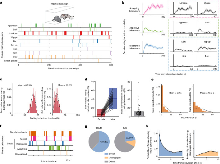
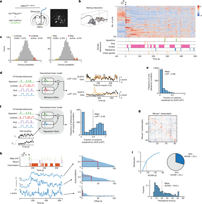
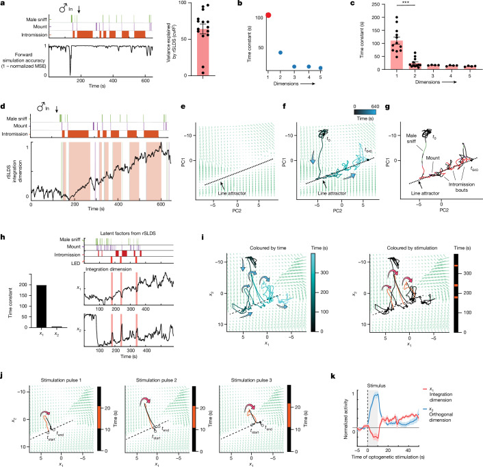
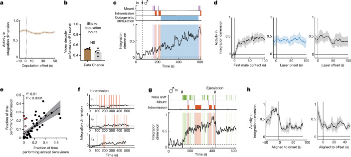
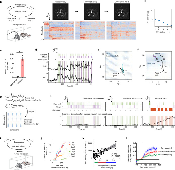
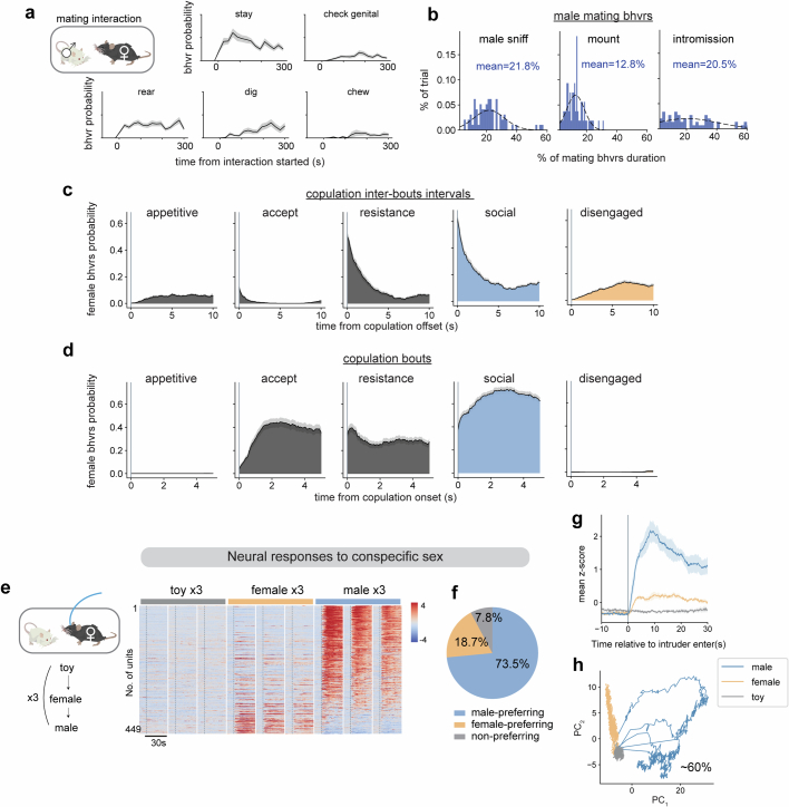
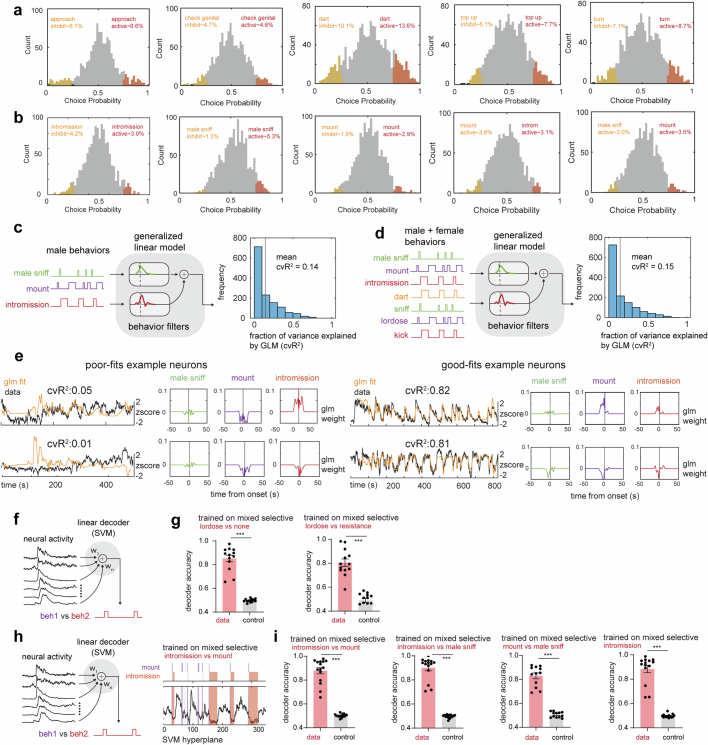
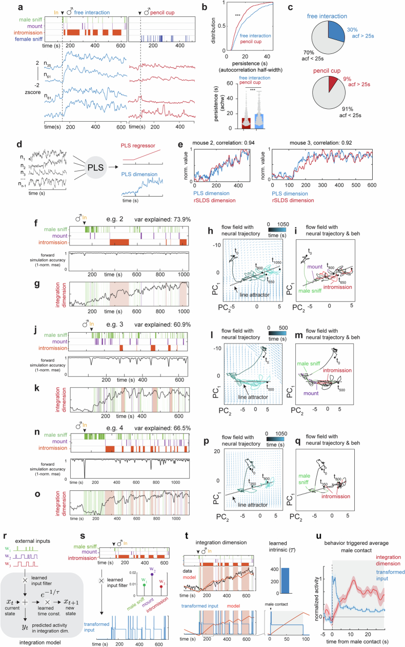
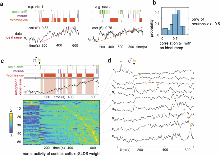
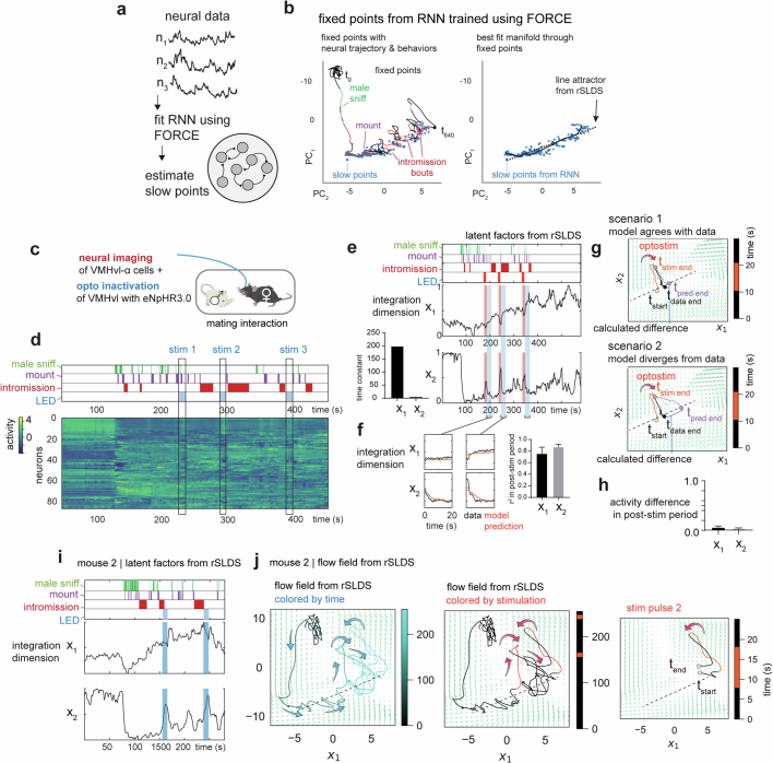
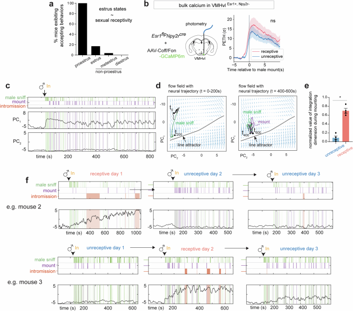
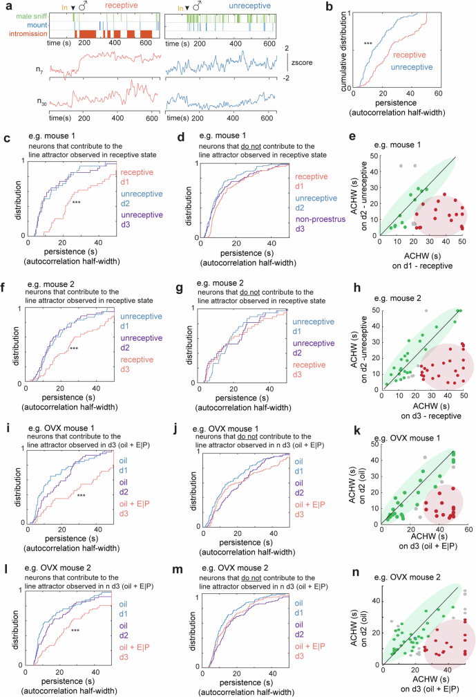
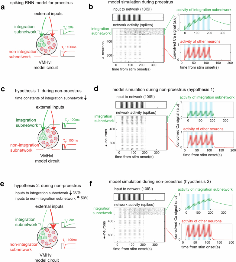
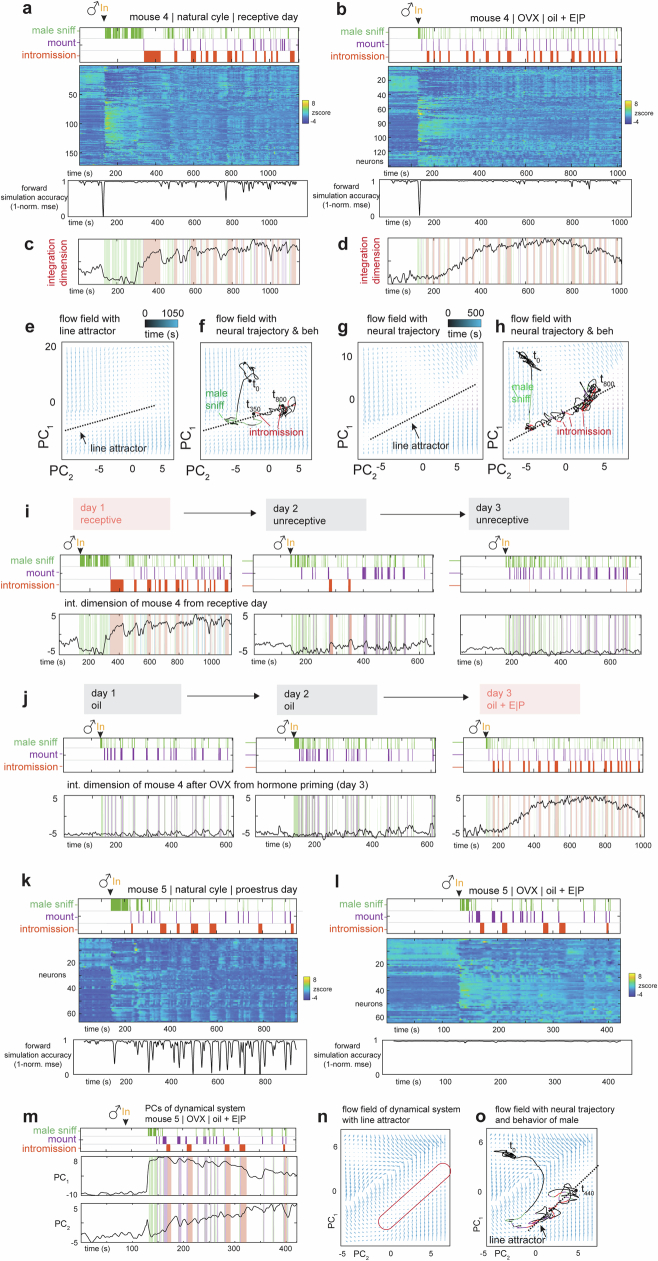
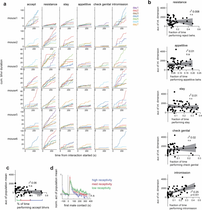
Females exhibit complex, dynamic behaviours during mating with variable sexual receptivity depending on hormonal status^1-4. However, how their brains encode the dynamics of mating and receptivity remains largely unknown. The ventromedial hypothalamus, ventrolateral subdivision contains oestrogen receptor type 1-positive neurons that control mating receptivity in female mice^5,6. Here, unsupervised dynamical system analysis of calcium imaging data from these neurons during mating uncovered a dimension with slow ramping activity, generating a line attractor in neural state space. Neural perturbations in behaving females demonstrated relaxation of population activity back into the attractor. During mating, population activity integrated male cues to ramp up along this attractor, peaking just before ejaculation. Activity in the attractor dimension was positively correlated with the degree of receptivity. Longitudinal imaging revealed that attractor dynamics appear and disappear across the oestrus cycle and are hormone dependent. These observations suggest that a hypothalamic line attractor encodes a persistent, escalating state of female sexual arousal or drive during mating. They also demonstrate that attractors can be reversibly modulated by hormonal status, on a timescale of days.

Fig. 1. Dynamics of female behaviours during mating interaction.

a, Raster plot of ten female mating behaviours during one interaction with a male. b, The probability of mating behaviours during every 20 s (n = 74 trials, n = 28 mice). Behaviours were grouped as accept (comprising lordose and wiggle), appetitive (comprising approach and sniff) and resistance (comprising dart, top up, kick and turn); data are presented as mean ± s.e.m. c, Distribution of the percentage of time females displayed responsive versus self-initiated mating behaviours over the total mating behaviour time in each trial (n = 74 trials). Female self-initiated mating behaviours comprised appetitive behaviours and check genital area. Female-responsive mating behaviours comprised accept and resistance behaviours and staying. d, Percentage of time female or male mice displayed self-initiated mating behaviours in each trial (left). The box boundaries range from minimum to maximum, with a line at the median. Male self-initiated mating time over female in each trial (right; n = 74 trials). Data are presented as mean ± s.e.m. Male self-initiated mating behaviours included male sniffing, mounting and intromission. e, Distribution of the durations of male copulation bouts (left; n = 1,685) and IBIs (right; n = 1,611). Male copulation included mounting and intromission. f, Raster plot of female behaviours during copulation bouts and IBIs. Social behaviours comprised accepting, resistance and appetitive behaviours; and non-social disengaged behaviours comprised rearing, digging and chewing. g, Percentage of time females displayed social behaviours in each male copulation bout or IBI. ‘Others’ indicates all behaviours other than the defined social behaviours or non-social disengaged behaviours during interaction. h, Female behaviour probability aligned to male copulation offsets.

Fig. 2. Tuning properties of female VMHvl neurons during mating.

a, Schematic of the miniscope imaging of female VMHvl^{Esr1+,Npy2r−} α-cells (left), and an example imaging plane (right). b, Diagram showing the mating interaction test. Single-cell responses during the mating interaction (top right) and their corresponding behaviours (bottom right), from one example female are shown. Units were sorted by temporal correlation. The colour scale indicates z-scored activity. c, Choice probability histograms and the percentages of tuned cells. Cut-off of choice probability > 0.7 or choice probability < 0.3 and more than 2σ (n = 15 mice). d, Schematic showing the GLM used to predict neural activity from behaviour (left), and an example fit of selected neurons with cvR² (right; 0.50 and 0.01). e,f, Distribution of cvR² across all mice for GLMs trained using only behaviour (e; n = 15 mice) and using behaviour with cell coupling (f; n = 15 mice). g, Predicted cell coupling (relative strength of connectivity) between neurons in one example mouse. h, Example VMHvl neurons in female mice showing a range of persistent activity (left; z-scored ∆F/F), and the ACHW as a measure of persistent activity for example units shown (right). The red rectangle highlights the autocorrelation half-width, which is measured by finding the offset value (in seconds) that relates to an autocorrelation of 0.5. i, Cumulative distribution of ACHW for all units (top), and distribution of the number of neurons with ACHW > 25 s (bottom; n = 4 mice).

Fig. 3. An approximate line attractor in female VMHvl during mating.

a, rSLDS model performance measured by forward simulation accuracy (calculated as (1 − normalized mean squared error (MSE)) in an example mouse (left), and variance explained by a rSLDS model fit without an input term (Methods) for all mice (right; n = 15 mice, mean = 64.08%). The variance explained by the two outliers can be increased by incorporating an input term. b, Time constants reveal a single dimension with a large time constant. c, Distribution of time constants across animals fit by the rSLDS. Time constants are sorted by magnitude in each animal (***P < 0.001; n = 15 mice; mean time constant of dimension 1: 110.7 ± 13.6 and dimension 2: 24.5 ± 5.1; P = 6.5 × 10⁻⁵). d, Dynamics of the integration dimension reveals a ramping dimension, aligned to male mating behaviours in an example trial. Variance explained of 73.7%. e, Flow field of VMHvl α-cell dynamical system. PC1 principal component 1. f, Flow field of VMHvl α-cell dynamical system showing neural trajectories in state space. t₀, time 0 s. g, Neural state space of VMHvl α-cell dynamical system and behaviours, highlighting regions where fixed points are present (dashed line). h, Time constants of latent factors from the rSLDS model (left), and projection of rSLDS latent factor activity from the rSLDS model trained on neural data from unperturbed periods (right; that is, excluding LED stimulation and 20-s post-stimulation interval). i, Flow field and neural trajectories from the rSLDS model coloured by time (left), and neural trajectory coloured by stimulation periods (right). j, Flow field and neural trajectories for each of the three stimulation periods for mouse 1. Note that trajectories are pushed away from the attractor during stimulation and then return to the line attractor following stimulation offset, as predicted by the flow field. This approach also tests the validity of the extrapolated regions of the flow field uncovered by the rSLDS. k, Stimulus-triggered average of response in integration dimension (x₁) and orthogonal dimension (x₂) upon optogenetic stimulation. n = 3 mice. The dotted vertical line indicates the onset of the stimulus, and the shaded area represents the duration of the stimulus. The horizontal line indicates the pre-stimulus baseline of normalized activity.

Fig. 4. A line attractor encodes a persistent and ramping state during mating.

a, Behaviour-triggered average of the normalized activity of the integration dimension aligned to the offset of male copulation. Dashed line represents offset of copulation events. Data are presented as mean ± s.e.m. b, Videoframe behavioural decoder performance trained on neural data from copulation bouts versus IBIs (n = 4 mice, P = 0.2, Mann–Whitney U-test, mean value of data of 0.52 ± 0.007, shuffle of 0.49 ± 0.03). c, Dynamics of the integration dimension in an example female combined with optogenetic inhibition of mating behaviours in the interacting male. d, Behaviour-triggered average of the normalized activity of the integration dimension aligned to first male contact (left), optogenetic mating inhibition onset (middle) and inhibition offset (right; n = 4 mice). Data are presented as mean ± s.e.m. e, Scatter plots of time spent by males performing intromission and time spent by females performing acceptance behaviours to identify trials with high intromission and low receptivity (coloured dots). Data are presented as mean ± s.e.m. P = 7.09 × 10⁻¹². f, Example traces of the integration dimension for trials with intromission but low receptivity (identified from panel e). g, Dynamics of the integration dimension, aligned to male mating behaviours in an example trial with ejaculation. h, Behaviour-triggered average of the normalized activity of the integration dimension aligned to the ejaculation onset and offset (n = 4 mice). Data are presented as mean ± s.e.m. Dashed line indicates the onset or offset of ejaculation.

Fig. 5. Female line-attractor dynamics encoded sexual receptivity across days.

a, Illustration of the longitudinal imaging strategy across oestrus states of naturally cycling female mice (left), and example longitudinal imaging planes and traces from one female (right). Units were sorted by temporal correlation. The colour scale indicates z-scored activity. b, Time constants of the VMHvl α-cell dynamical system on 1 unreceptive day. c, Line-attractor scores for dynamical systems fit during receptive and unreceptive days (n = 4 mice, mean ± s.e.m. of 0.05 ± 0.02 (unreceptive) and 1.9 ± 0.2 (receptive); *P < 0.05, Mann–Whitney U-test, P = 0.02). d, Low-dimensional principal components of a VMHvl α-cell rSLDS fit model on a unreceptive day. Principal components show fast time-locked dynamics and lack ramping and persistence. e, Flow field of the VMHvl α-cell dynamical system on an unreceptive day. f, Same as panel e, but showing neural trajectories in the state space coloured by time and behaviours. g, Schematic showing the projection of neural activity from an unreceptive day into the fit dynamical system from a receptive day. h, Dynamics of integration dimension in the VMHvl discovered during a receptive day (same example trial as shown in Fig. 3d) compared with activity of the same dimension on unreceptive days. i, Illustration of the longitudinal imaging strategy across oestrus states of naturally cycling females with oestrogen injection. j, Accepting behaviours displayed in mating interactions across days from one example female. k, Scatter plots of the integration dimension values and the amount of female accepting behaviours (n = 50 trials) in each trials. Data are presented as mean ± s.e.m. l, The integration dimension activity aligned to the first male contact, in high-receptivity, medium-receptivity or low-receptivity trials, as defined in k. ****P < 0.0001, Wilcoxon matched-pairs signed-rank test. Data are presented as mean ± s.e.m.

Extended Data Fig. 1. Behavior dynamics and neural responses to conspecific sex.

a, The probability of female behaviors every 20 s (n = 74 trials, N = 28 mice). b, Distribution of the percentage of time males displayed mating behaviors in each trial (n = 74 trials). c, The probability of female behaviors aligned to male copulation offsets and d, copulation onsets. (e-h), Neural responses to conspecific sex. e, Left, diagram of sex representation test. Each intruder was presented for 1 min. Right, concatenated average responses to toy, female, or male (N = 8 mice). Color scale indicates z-scored activity. Units were sorted by temporal correlation. f, Percentages of male- or female-preferring cells (calculated by Choice Probability). g, Mean responses of female VMHvl^Esr1 α cells to male, female and toy (N = 8 mice). Data presented as mean ± SEM. h, PCA of neuronal responses to male, female and toy from one example female.

Extended Data Fig. 2. Neural tuning to conspecific sex and behavior.

a, Choice Probability (CP) histograms and percentages of tuned cells for female behaviors. cutoff: CP > 0.7 or <0.3 and >2σ. N = 15 mice. b, Same as a, but for male behavior. c, Schematic showing generalized linear model (GLM) used to predict neural activity from male behaviors and distribution of cvR² across all mice, or d, both male and female behaviors and distribution of cvR² across all mice (N = 15 mice). e, Example generalized linear model fits and behavior filters for poorly and well fit neurons. (f-i), Decoder analysis. f, schematic showing linear support vector machine (SVM) decoder trained on frames of male mating behaviors. g, performance of the decoder trained to separate female behavior. Left, performance of decoder trained to separate frames of lordosis versus all remaining frames (***p < 0.001, N = 15 mice, mean decoder performance data: 0.85 ± 0.03, shuffle: 0.49 ± 0.003). Right, performance of decoder trained to separate frames of lordosis versus resistance behaviors (***p < 0.001, N = 15 mice, mean decoder performance data: 0.80 ± 0.03, shuffle: 0.48 ± 0.01). h, Same as f, but showing the decoder hyperplane for separating male behaviors (mount versus intromission) on right. (***p < 0.001). (N = 15 mice). i, performance of decoders trained to separate intromission versus mount (mean decoder performance data: 0.89 ± 0.02, shuffle: 0.49 ± 0.003), intromission versus male sniffing (mean decoder performance data: 0.90 ± 0.02, shuffle: 0.49 ± 0.003), mount versus male sniffing (mean decoder performance data: 0.83 ± 0.02, shuffle: 0.50 ± 0.006) and intromission versus remaining frames male sniffing (***p < 0.001, N = 15 mice, mean decoder performance data: 0.88 ± 0.03, shuffle: 0.48 ± 0.003).

Extended Data Fig. 3. Additional example trials with rSLDS model fit, additional information for Fig. 3.

a, Dynamics of persistently active neurons identified during receptive interaction with pencil-cup assay. b, Cumulative distribution & bar plot of ACHW for same neurons during free interaction vs pencil cup assay ****p < 0.0001, Mann-Whitney U test, p value: 1.25e-11, N = 470 neurons from 5 mice. mean ACHW during pencil cup: 14.3 ± 0.42, free interaction: 19.6 ± 0.58. c, Pie chart indicating fraction of neurons with ACHW > 25 s in free interaction and in pencil cup assay. d, Schematic illustrating partial least squares regression to extract integration dynamics in VMHvl. e, Comparison of rSLDS integration dimension and PLS dimension for two example mice showing a high correlation. (f-q), Additional example trials with rSLDS model fit. f, Recurrent switching linear dynamical systems (rSLDS) model fit forward simulation accuracy aligned to male behaviors in example trial 2. g, Dynamics of the integration dimension in trial 2. h, Flow field of VMHvl α dynamical system showing neural trajectories in state space, annotated by time from male encounter (t₀) for trial 2. i, Neural state space of VMHvl α dynamical system highlighting behaviors and the region containing the line attractor for trial 2. j-m, the same as g-i for example trial 3. n-q, the same as j-i for example trial 4. r, Integration model used to dissect the contribution of intrinsic decay and external inputs (male behaviors; male-sniff, mount, and intromission). A single state LDS model is used to fit external inputs to predict activity in the integration dimension. s, Top: External inputs to integration model, middle: learned input filter showing weights that are multiplied with the external inputs. Bottom: transformed input obtained by multiplying external inputs with input filter. t, Top: Data and model prediction from LDS to predict activity in the integration dimension. The learned model has a large intrinsic time constant (right). Bottom: Transformed input (weighted input from three male behaviors) and model prediction overlayed with behaviors. u, Behavior triggered average of transformed input and integration dimension aligned to male contact. Male contact is present for the duration of the shaded region. Data presented as mean ± SEM.

Extended Data Fig. 4. Dynamics of single cell activity.

a, Correlation of example unit activity with an ideal ramp. b, Distribution of correlation of individual neuron activity with ideal ramp. c, Upper, relationship of male behavior to weighted average of all units contributing to integration dimension as a function of time. Data from the same example trial as shown in Fig. 3d. Lower, normalized activity (z-score) of individual units times rSLDS weight for each unit exhibiting a significant weight in the integration dimension, sorted by time to peak. d, Traces of example units from c, lower. Yellow arrow indicates peak of activity for each unit.

Extended Data Fig. 5. Independent verification and neural perturbations of line attractor dynamics.

a, Cartoon illustrating approach of fitting RNNs to neural data using FORCE. b, Slow points and attractor manifold uncovered by FORCE, overlaid with line attractor uncovered by rSLDS. c, Paradigm for simultaneous neural perturbation & imaging during a mating interaction in females. GcaMP was expressed in VMHvl-α cells while halorhodopsin (eNpHR3.0) was expressed in all VMHvl neuron using a pan-neuronal driver. d, Neural data obtained from a female showing annotated male behaviors and optogenetic inhibition (LED). e, Left: Latent factors from two-dimensional rSLDS model fit to neural data. Reproduced for explanatory purposes from Fig. 3h. Right: Time constants of the two longest-lived dimensions from rSLDS model fit to data from unperturbed periods (excluding stimulation period plus a 20 s post-stimulus period). f, Left: Performance of model on held out data from 20 s immediate post-stimulus period (taken from highlighted blue portions of graphs in e). g, Cartoon depicting quantification of flow field prediction following optogenetic perturbation. The flow field fit from unperturbed periods of time is used to predict the neural trajectory following perturbation (t-pred end, purple line). This trajectory is then compared to data (t-data end, black line). Scenario 1 illustrates when the model agrees with data, resulting in a low difference in activity along the line attractor (top). Scenario 2 illustrates when the model diverges from data resulting in a large deviation in final position along the line attractor (bottom). h, Quantification of flow field prediction following perturbation as the difference in activity level at the end of the 20 s post-stimulus period between data and model in both x1 and x2 dimensions across mice (activity difference for x1: 0.05 ± 0.03, for x2: 0.03 ± 0.01, n = 3 mice). i, Latent factors from rSLDS of mouse 2 during neural perturbation. j, Flow field and neural trajectories for mouse 2. Note that trajectories are pushed away from the attractor during stimulation and then return to line attractor following stimulation offset, as predicted by the flow field.

Extended Data Fig. 6. Line attractor dynamics across the estrus cycle.

a, Correlation between female estrus states and the presence of sexual receptivity, measured by whether female displayed accepting behaviors during interaction with male. b, Photometry recording in female VMHvl α cells during receptive and unreceptive mating interactions. Data presented as mean ± SEM. c, Low dimensional principal components of VMHvl α dynamical system in receptive day with neural data projected from unreceptive day. d, Flow field of VMHvl α dynamical system in receptive day with neural trajectories projected from unreceptive for t = 0 to t = 200 s (left) and t = 200 s to t = 400 s (right). e, Quantification of normalized value of integration dimension during male-mounting in unreceptive and receptive days (*p < 0.05, N = 4 mice, mean value during unreceptive day: 0.09 ± 0.04, receptive day: 0.69 ± 0.05. Mann-Whitney U test, p value: 0.02). f, Dynamics of integration dimension in two more example mice discovered during receptive day compared to activity of the same dimension on unreceptive days.

Extended Data Fig. 7. Single cell persistence at receptive and unreceptive days.

a, Example units active during both receptive (red traces, left) and unreceptive (blue traces, right), showing persistence on receptive day and fast dynamics on the unreceptive days. b, Comparison of cumulative distribution of ACHWs to that of same neurons on unreceptive days. Data from example mouse 1. ***p < 0.001, KS-test. c, Cumulative distribution of ACHWs for units with significant weights on integration dimension across receptive and unreceptive day, ***p < 0.001, KS-test. Data from example mouse 1. d, Cumulative distribution of ACHWs for example mouse 1, for units that do not contribute to the integration dimension on the receptive day, compared on receptive vs unreceptive days. e, Scatter plot of ACHWs for units with significant weights on integration dimension for receptive day vs unreceptive day. Data from example mouse 1. (f-h) Same as c-e for example mouse 2. i, Cumulative distribution of ACHWs for units with significant weights on integration dimension across hormone primed (day 3) and non-primed days (days 2, 1). ***p < 0.001, KS-test. Data from example OVX mouse 1. ***p < 0.001, KS-test. j, Cumulative distribution of AHWs for example OVX mouse 1, for units that do not contribute to the integration dimension across hormone primed (day 3) and non-primed days (days 2, 1). k, Scatter plot of ACHWs for units with significant weights on integration dimension for hormone-primed day vs non-primed day. Data from example OVX mouse 1 (l-n) Same as i-k. for example OVX mouse 2.

Extended Data Fig. 8. Mechanistic model for loss of line attractor dynamics in unreceptive states.

a, Schematic illustrating the construction of a spiking recurrent neural network (RNN) with a line attractor. The line attractor is created by allowing a subset of neurons to possess a larger intrinsic time constant (20 s vs 100 ms), and by denser connectivity within the subnetwork (12% versus 1% in remaining network). b, Model simulation during the proestrus phase with pulse like input delivered at 10 s ISI. Right, activity of integration subnetwork (green) and other neurons (red). c, Schematic for hypothesis 1: we hypothesize that during non-proestrus, there is a reduction in the intrinsic constant of the integration subnetwork (from 20 s to 100 ms). d, Same as b but for hypothesis 1 during non-proestrus. e, Schematic for hypothesis 2: we test whether changes in the firing rate of different neuronal subsets can lead to the loss of attractor dynamics. To investigate this, we provide the integration subnetwork with 50% reduced input strength, while increasing the same for the remaining neurons. f, Same as b but for hypothesis 2 during non-proestrus.

Extended Data Fig. 9. Population dynamics before and after OVX in the same female.

(a, b,) Neural raster and behaviors and rSLDS model performance (measured as forward simulation error, see Methods) for one example mouse in receptive day of natural estrus cycle a, and same mouse on hormone primed day after OVX (day3, oil + E | P) b. (c, d), Integration dimension identified by rSLDS on natural cycle receptive day c, and during hormone primed day after OVX d. (e, f), Flow field e, and neural trajectories of dynamical system f, with line attractor highlighted of model fit during the receptive state of the estrus cycle. (g, h), Same as e, f, for model fit during hormone primed day after OVX. i, Dynamics of integration dimension discovered during natural cycle receptive day compared to activity of the same dimension on unreceptive days. j, Dynamics of integration dimension in the same mouse discovered during hormone primed day (day 3) compared to the activity of the same dimension during non-primed days. (k, l), Neural raster and behaviors and rSLDS model performance for mouse in proestrus day of natural estrus cycle k, and same mouse on hormone primed day after OVX (day3, oil + E | P) l. m, Principal components of mouse dynamic system fit during hormone primed day. (n, o), Flow field n, and neural trajectories of dynamical system. o, with line attractor highlighted of model fit during the hormone primed day after OVX in mouse.

Extended Data Fig. 10. Longitudinal mating assay and correlation with attractor dynamics.

a, Behaviors displayed in mating interactions across days from all the recorded females. b, The scatter plots of the integration dimension values and the amount of female resistance behaviors (linear regression, R² = 0.008), appetitive behaviors (R² = 0.01), staying (R² = 0.01), checking genital (R² = 0.02) and male intromission (R² = 0.25). Data presented as mean ± SEM. c, correlation of area under the curve (auc) of the population mean of all neurons with the percentage of time spent performing accepting behaviors. Data presented as mean ± SEM. d: activity of population mean from trials with varying degrees of receptivity defined in a). Data presented as mean ± SEM, Mann-Whitney U test.

References

1. Jennings, K. J. & de Lecea, L. Neural and hormonal control of sexual behavior. Endocrinology161, bqaa150 (2020). - PMC - PubMed
1. Gutierrez-Castellanos, N., Husain, B. F. A., Dias, I. C. & Lima, S. Q. Neural and behavioral plasticity across the female reproductive cycle. Trends Endocrinol. Metab.10.1016/j.tem.2022.09.001 (2022). - PubMed
1. Yin, L. & Lin, D. Neural control of female sexual behaviors. Horm. Behav.151, 105339 (2023). - PMC - PubMed
1. Lenschow, C. & Lima, S. Q. In the mood for sex: neural circuits for reproduction. Curr. Opin. Neurobiol.60, 155–168 (2020). - PubMed
1. Liu, M., Kim, D.-W., Zeng, H. & Anderson, D. J. Make war not love: the neural substrate underlying a state-dependent switch in female social behavior. Neuron110, 841–856.e6 (2022). - PMC - PubMed
LinkOut - more resources