Abstract representations emerge in human hippocampal neurons during inference

Abstract

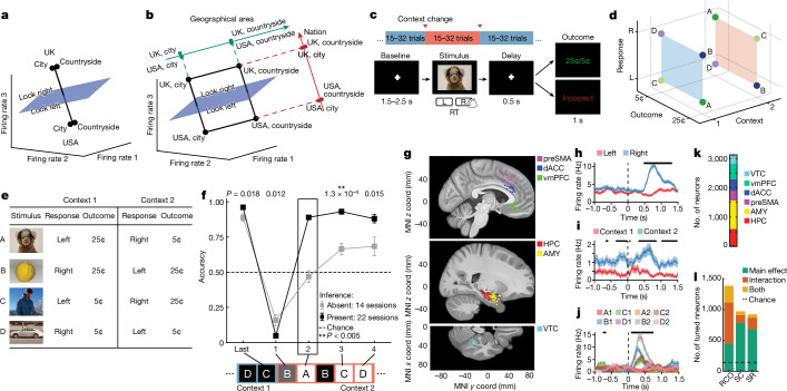
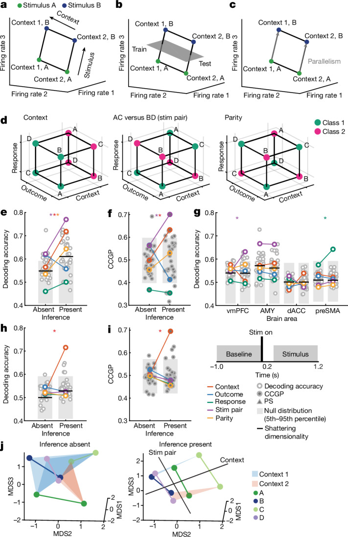
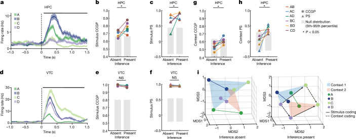
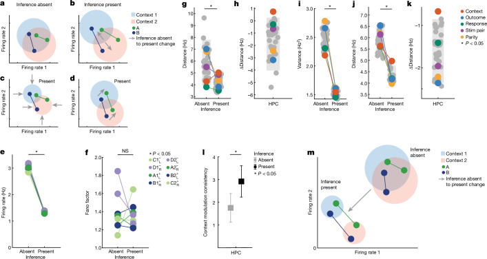
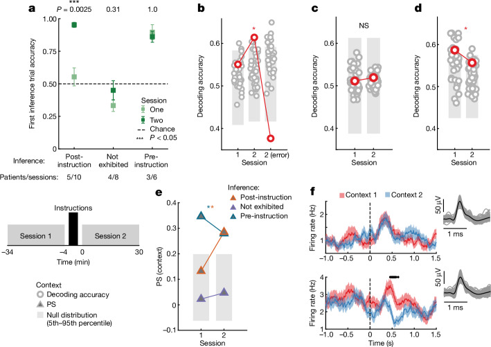
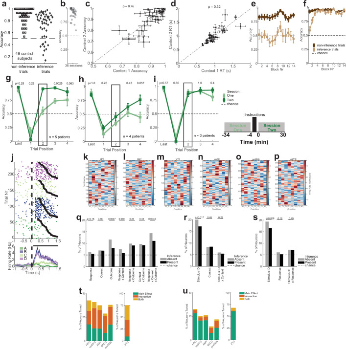
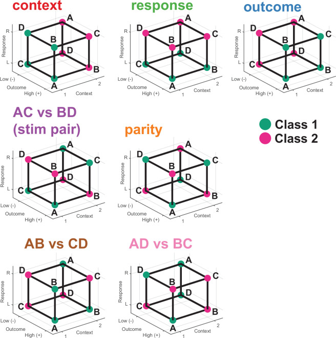
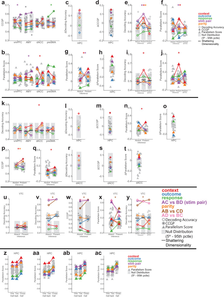
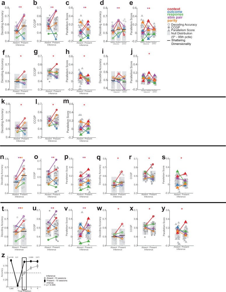
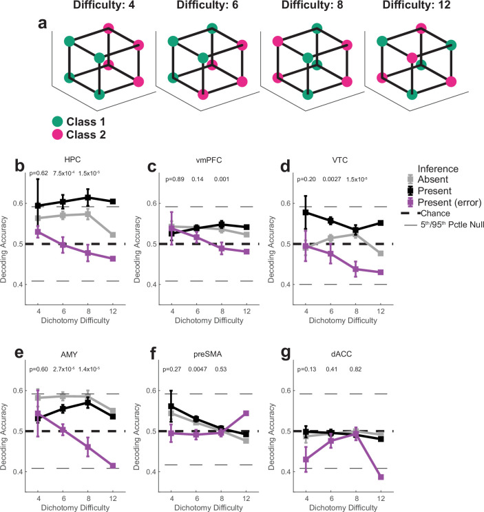
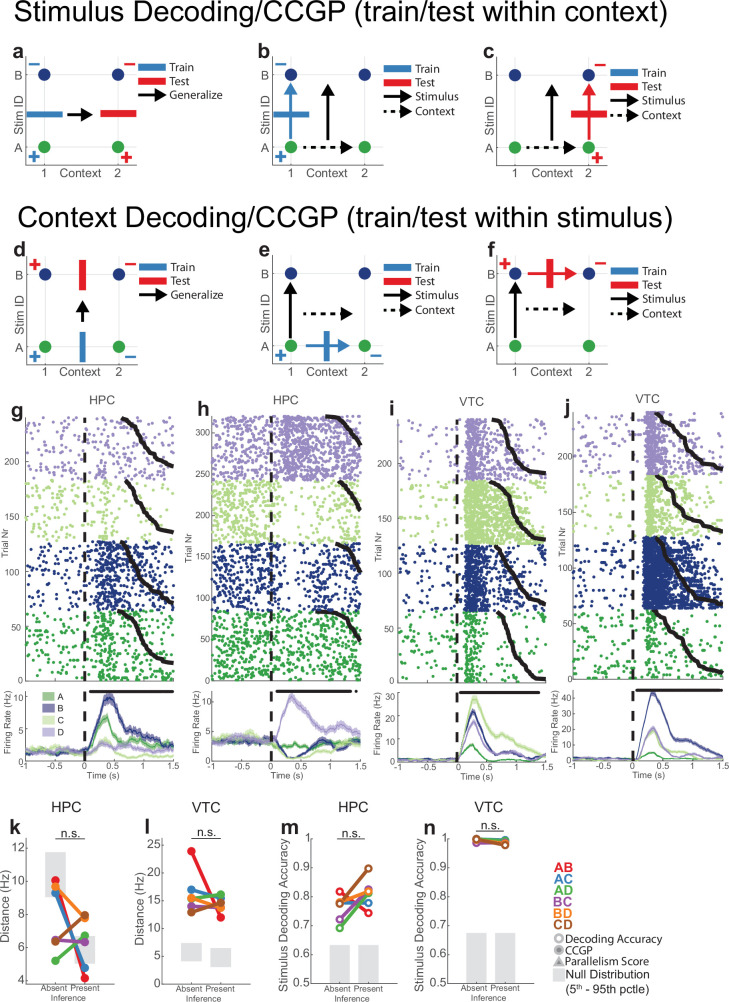
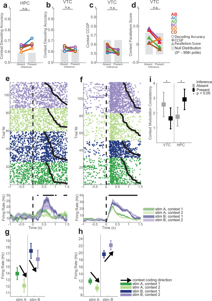
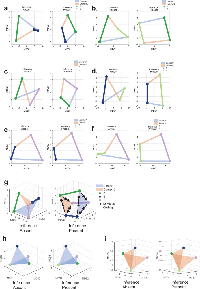
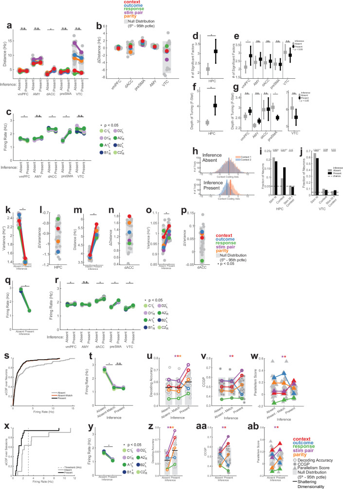
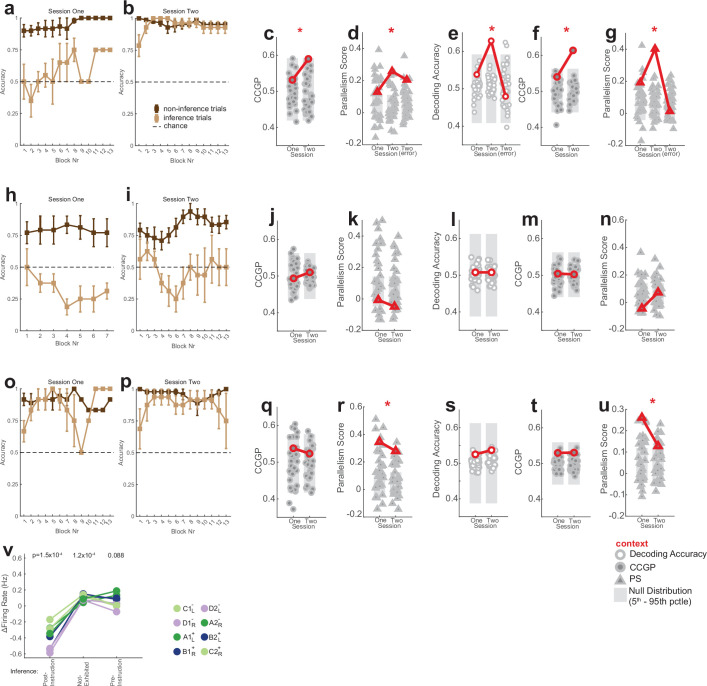
Humans have the remarkable cognitive capacity to rapidly adapt to changing environments. Central to this capacity is the ability to form high-level, abstract representations that take advantage of regularities in the world to support generalization¹. However, little is known about how these representations are encoded in populations of neurons, how they emerge through learning and how they relate to behaviour^2,3. Here we characterized the representational geometry of populations of neurons (single units) recorded in the hippocampus, amygdala, medial frontal cortex and ventral temporal cortex of neurosurgical patients performing an inferential reasoning task. We found that only the neural representations formed in the hippocampus simultaneously encode several task variables in an abstract, or disentangled, format. This representational geometry is uniquely observed after patients learn to perform inference, and consists of disentangled directly observable and discovered latent task variables. Learning to perform inference by trial and error or through verbal instructions led to the formation of hippocampal representations with similar geometric properties. The observed relation between representational format and inference behaviour suggests that abstract and disentangled representational geometries are important for complex cognition.

Fig. 1. Task, behaviour and single-neuron tuning.

a,b, Possible definitions of abstraction as clustering (a) or generalization (b). In the latter, the two variables are orthogonal to each other and preserved, whereas one of the variables (geographic area) is discarded in the former. c, Task and example trial. Blocks of trials alternated between the two contexts. In each trial, the stimulus remained on the screen until participants pressed a button, followed by the outcome. d,e, Task structure. d, Each stimulus (A–D) is associated with a single correct response and results in either a high or low reward if the correct response is given. e, Stimulus–response relationships are inverted between contexts 1 and 2. f, Behaviour. Accuracy is shown separately for inference present (n = 22) and absent (n = 14) sessions for the last trial before the context switch, the first trial after the context switch and for the remaining three inference trials averaged over all trials in each session (mean ± s.e.m. across sessions). The dashed line marks chance. The black box indicates inference trial 1. **P < 0.005 for rank-sum inference sbsent versus present over sessions. g, Electrode locations. Each dot denotes a microwire bundle. Locations are shown on the same hemisphere (right) for visualization purposes only. h–j, Example neurons that encode response (h), context (i) and mixtures of stimulus ID (indicated by A–D) and context (indicated by 1 or 2) (j). Error bars are ± s.e.m. across trials. t = 0 is stimulus onset. Black points indicate P < 0.05 of one-way ANOVA of plotted variables. k, Number of units recorded in each brain area. l, Number of single units across all brain areas showing significant main or interaction effects to at least one variable (n-way ANOVA, P < 0.05, Methods). Variables tested: response (R), context (C), outcome (O), and stimulus ID (S). Brain areas assessed: amygdala (AMY), dorsal anterior cingulate cortex (dACC), hippocampu (HPC), presupplementary motor area (preSMA), and ventromedial prefrontal cortex (vmPFC).

Fig. 2. Multiple abstract variables emerge with inference in hippocampus.

a, Example neural state space formed by three neurons. Points represent the response patterns in various task conditions. Black arrows mark coding vectors. b, CCGP. A decoder is trained to differentiate between stimulus A and B in context 1 and evaluated in context 2. If context is represented in an abstract format, then the decoder generalizes, yielding high CCGP for context. c, PS. In disentangled representations, the coding vectors (arrows) are parallel. d, Illustration of the dichotomies (variables) context, stim pair and parity with class labels indicated. See Extended Data Fig. 2 for all dichotomies. e,f, Neural representation during stimulus period in hippocampus. Context and stim pair are decodable in inference present sessions (e) and are encoded in an abstract format (f). Each dot shows one of the 35 dichotomies. The horizontal black line shows shattering dimensionality. Grey bars denote the 5th–95th percentile of the null distribution. Stars denote named dichotomies that are above chance in inference present sessions and are significantly different from their corresponding inference absent value (P_RS < 0.05/35, two-sided rank-sum test, Bonferroni corrected for multiple comparisons across all dichotomies). g, Decodability of all dichotomies for the other brain areas. AMY, amygdala. See e for notation. h,i, Neural representation during baseline period in hippocampus is decodable in inference present (h) and encoded in an abstract format (i). Trials are labelled according to the previous trial. See e,f for notation. Context differed significantly between present and absent (P = 1.1 × 10⁻³³ and P = 2.4 × 10⁻³⁴, respectively). j, Hippocampal population response during the stimulus period in inference absent and present sessions shown using MDS (Methods). Points correspond to stimuli and context combinations, black lines show hypothetical hyperplanes for context and stimulus pair decoders. In all panels, neuron counts are balanced between inference absent and inference present sessions for every brain area to make values comparable. *P < 0.05.

Fig. 3. Stimulus representations become structured around context with inference in hippocampus but not VTC.

a–f, Encoding of stimulus identity across contexts. a–c, Responses in hippocampus (HPC) following stimulus onset carry information about stimulus identity. a, Example hippocampal neuron encoding stimulus identity. b,c, Representational geometry of stimulus identity across contexts. Analysis is conducted over pairs of stimuli in each context (legend). Significance of differences is tested using a two-sided rank-sum test comparing inference absent and present over all stimulus pairs (*P < 0.05, NS otherwise). All other conventions identical to those in Fig. 2. b,c, CCGP (P_RS = 0.041) (b) and PS (P_RS = 0.040) (c) for stimulus coding across contexts significantly increased in inference present compared to inference absent sessions. d–f, Responses in VTC following stimulus onset carry information about stimulus identity. d, Example VTC neuron encoding stimulus identity. e,f, CCGP (P_RS = 0.15) (e) and PS (P_RS = 0.39) (f) for stimulus coding across contexts does not differ significantly between inference absent and inference present sessions. g,h, Same analysis as in a–f, but for encoding of context across stimulus pairs for hippocampus (see b,c for plotting conventions). CCGP (P_RS = 0.012) (g) and PS for context coding vectors between pairs of stimuli (P_RS = 0.015) (h) both significantly increase from inference absent to inference present sessions. i, Summary of changes in neural geometry in hippocampus. Shown is the MDS of condition-averaged responses of all recorded neurons shown for inference absent and present sessions. Points are average population vector responses to combinations of stimuli and context. Lines connect the same stimuli across context. Abstract coding of stimulus across contexts (solid arrows) and context across stimuli (dashed arrows) are highlighted for one pair of stimuli (C and D). The data in this plot are identical to those of Fig. 2j. Error bars in a,d are ±s.e.m. across trials. All P_RS values are from a two-sided rank-sum test.

Fig. 4. Firing-rate properties underlying the emergence of abstract variables in the hippocampus.

a–d, Changes that could give rise to abstract variables. Shaded circles represent variability, and grey arrows signify changes between inference absent and present. a, Original, when variable is not abstract. b, Increase in distance. c, Decrease in variance. d, Increase in parallelism. e, Firing rates of hippocampal neurons during stimulus period decreased (P_RS = 8.3 × 10⁻⁵, two-sided rank-sum over conditions). Colour indicates task state, with coding indicating identity (for example, task condition C1⁻_L describes stimulus C, context 1, outcome $-$, response L). f, Fano factor was not significantly different between inference present and absent sessions (two-sided rank-sum test, P_RS = 0.99). g, Population distance between centroids for all 35 balanced dichotomies. Average distances decrease from inference absent to present (P_RS = 2.9 × 10⁻⁸, rank-sum over dichotomies). Grey bars indicate the 5th–95th percentile of the geometric null distribution. h, Context alone is the only dichotomy whose distance significantly increases from inference absent to present (red, P_ΔDist = 0.040, against geometric null of difference). HPC, hippocampus. i, Average trial-by-trial variance projected along the coding direction decreased on average between inference absent and inference present sessions (P_RS = 6.5 × 10⁻¹³, rank-sum test). j,k, Same as g,h, but for spike counts during the baseline period. Trials are grouped by identify the previous trial. Distance was significantly reduced across all dichotomies (j, P_RS = 6.4 × 10⁻¹³, rank-sum over dichotomies) and context alone shows a distance reduction that is smaller than would be expected by chance (k, red, P_ΔDist = 0.027, against geometric null of difference). l, Stimulus-tuned neurons in the hippocampus were modulated by context more consistently in inference present sessions (P_RS = 0.0039) during the stimulus period (n = 63, error bars are ±s.e.m. across neurons). m, Illustration of changes in neural state space. Context dichotomy distance increased, variance decreased and consistency of stimulus modulation across contexts increased. In all panels, P_RS values are from a two-sided rank-sum test and grey bars indicate the 5th–95th percentile of the geometric null distribution.

Fig. 5. Abstract hippocampal representation of context is present following successful verbal instructions.

a, Top, behavioural performance on the first inference trial for patients that performed inference after instructions (n = 10 sessions, post-instruction), those that did not perform inference even after instructions (n = 8 sessions, not exhibited) and those that performed inference already before instructions (n = 6 sessions, pre-instruction). Error bars are ±s.e.m. across sessions and P values are rank-sum session 1 versus 2. Bottom, schematic of the experiment. Session before and after high-level instructions are referred to as sessions 1 and 2, respectively. b–d, Encoding of context during the stimulus period in different groups of patients. The first trial following a switch is excluded from this analysis. *P < 0.05 against null in any column of a given geometric measure plot estimated empirically from the null distribution. b, Post-instruction group. Context was significantly decodable in session 2 correct but not error trials and also not in session 1 (P₁ = 0.17, P_1(correct) = 0.016, P_RS = 3.1 × 10⁻¹⁹, P_2(error) = 0.99). c, Not exhibited group. Context was not significantly decodable (P₁ = 0.44, P₂ = 0.42). d, Pre-instruction group. Context was decodable in session 1 (P₁ = 0.014, P_Two = 0.17). e, Summary of changes due in instructions based on the PS for context. Neuron counts are equalized across groups by subsampling. Context PS increases significantly from session 1 to 2 in the post-instruction group (P_{Postinstruction,i} = 0.20, P_{Postinstruction,2} = 0.0028). Context PS is not significantly different from chance for the not exhibited group (P_{Not exhibited,1/2} < 0.5) and is different from chance in both sessions for the pre-instruction inference (P_{Pre-instruction,1/2} < 0.005) group. All P values are versus chance and are empirically estimated from the null distribution. f, Example hippocampal neuron with univariate context encoding in the session after (bottom) but not before (top) instructions (one-way ANOVA, P_One = 0.40, P_Two = 0.010). Error bars are ±s.e.m. across trials.

Extended Data Fig. 1. Task behavior and single-neuron responses across all recorded regions.

(a) Task performance of n = 49 control subjects. Accuracy is reported as an average for each subject over all non-inference trials (left) and all inference trials (right; included are 3 the three trials after every switch in which an image was seen the first time after the switch, i.e. timepoints 2–4 in Fig. 1f). Chance is 50%. This task variant is equivalent to the first session of the task encountered by patients (before explicit instructions of latent task structure). 46/49 subjects performing above chance on non-inference trials. (b) Performance of patients in non-inference trials. Each dot is a single session. Only sessions where patients exhibited above-chance accuracy on non-inference trials are shown (36/42 sessions, p < 0.05, one-sided Binomial Test on all non-inference trials vs. 0.5). (c) Non-inference performance for context 1 and 2 for the n = 36 sessions included in the analysis. Error bars are SEM over blocks. The reported p-value is a paired two-sided t-test between the mean accuracies for Context 1 and Context 2 across all sessions. (d) Same as (c), but with reaction time (RT), computed as time from stimulus onset to button press for every trial. Mean RT’s are also computed by block. n = 36 sessions. (e-f) Performance as a function of time in the task for the (e) inference absence and (f) inference present groups. Shown is the accuracy for the last non-inference trial before a switch and the first inference trial after a switch. Accuracy is shown block-by-block averaged over a 3-block window (mean ± s.e.m. across sessions). (g-i) Behavioral performance for the subjects in the post-instruction, not-exhibited, and pre-instruction groups, respectively. See Fig. 1f for notation. Plot shows performance on the last trial before the context switch, the first trial after the context switch, and for the first inference trial (Trial 2) averaged over all trials in each session (mean ± s.e.m. across sessions). Dashed line marks chance. The first inference trial performance (block box) was used to classify patients the patients, so significance is not reported for this trial. P-values are a one-way binomial test vs. 0.5. (j) Example hippocampal neuron that encodes stimulus identity. Raster trials are reordered based on stimulus identity, and sorted by reaction time therein (black curves). Stimulus onset occurs at time 0. Black points above PSTH indicate times where 1-way ANOVA over the plotted task variables was significant (p < 0.05). Errorbars are ±s.e.m. across trials. (k-p) Normalized activity for all neurons recorded from the hippocampus (k), amygdala (l), VTC (m), dACC (n), preSMA (o), and vmPFC (p). Each is plotted as a heat map of trial-averaged responses to each unique condition (8 total, specified by unique Response-Context-Outcome combinations). Z-scored firing rates are computed from 0.2 s to 1.2 s after stimulus onset for every trial. Each row of the heat map corresponds to the activity of a single neuron, and columns correspond to each of the 8 conditions. Neurons are ordered such that adjacent rows (neurons) are maximally correlated in 8-dimensional condition response space. This approach would allow for modular tuning to visibly emerge in the heat map if groups of neurons were clustered in their response profiles. (q) Percentage of neurons across all areas that exhibit tuning. Tuning was assessed by fitting a 2 × 2 × 2 (Response-Context-Outcome) ANOVA for every individual neuron’s firing rate during a 1 s window during the stimulus presentation period. Significant neurons were counted as p < 0.05 for main effects or interaction effects involving the stated variables. Significanctly different proportions of tuned neurons between inference present and absent sessions is determined via a two-sided z-test, where “*” indicates p < 0.05, “***” indicates p < 0.005, and “n.s.” indicates “not significant”. (r) Same analysis as (q), but for a 4 × 2 ANOVA for stimulus identity and context. (s) Same analysis as (q), but for a 4 × 2 ANOVA for stimulus identity and response. (t) Percentages of tuned neurons shown separately for each region (compare to Fig. 1j). Single-neuron tuning is identified using a 3-Way ANOVA (Response × Context × Outcome), corresponding to column 1 (RCO) of Fig. 1j. (u) Same as (t), but single-neuron tuning identified here using 2-Way ANOVA (Stimulus ID × Context), corresponding to column 2 (SC) of Fig. 1j.

Extended Data Fig. 2. Visual representation of all named balanced dichotomies.

Illustration of the named balanced dichotomies that correspond to condition splits that have clearly interpretable meaning with respect to the construction of the task. For example, the context dichotomy (top left), arises from assigning all conditions for context = 1 to one class and all conditions for which context = 2 to the other class. The specific assignment of class labels 1 and 2 is arbitrary, and inverting the labels still corresponds to the same meaning for the dichotomy. All named dichotomies shown here are color coded to reflect their value in all Shattering Dimensionality, CCGP, and Parallelism Score plots, and this color code remains consistent throughout the paper whenever balanced dichotomies are considered.

Extended Data Fig. 3. Additional geometric analysis during stimulus processing and baseline periods.

(a) CCGP for other brain regions during stimulus period. See Fig. 2 for notation. Significant named dichotomies are marked when the dichotomies are above the 95^th percentile of the null distribution in inference present sessions and significantly different between inference absent and present (RankSum p < 0.01/35, Bonferroni corrected for balanced dichotomies). Significant increases were observed in vmPFC for stim pair (purple, p_Absent = 0.45, p_Present = 0.014) and preSMA for response (green, p_Absent = 0.045, p_Present = 0.0010) Stim pair CCGP in AMY was above chance for both inference absent and present sessions (purple, p_Absent = 0.050, p_Present = 0.039). (b) Same as (a), but for PS. PS increased significantly for stim pair in amygdala (purple, p_Absent = 1.3 × 10⁻⁴, p_Present = 9.0 × 10⁻⁸) and context in the dACC (red, p_Absent = 0.99, p_Present = 3.9 × 10⁻¹²). (c) Change in decoding accuracy. (d) Same as (c), but for CCGP. (e-f) Error trial analysis for neural response following stimulus onset in the hippocampus. Context (red) is not decodable and not in an abstract format in incorrect trials during inference present sessions. Only correct trials are used in inference absent sessions. Horizontal black bars indicate shattering dimensionality. Stars denote named dichotomies that are above chance in the inference present trials and are significantly different from their corresponding inference absent value (p < 0.05/35, Bonferroni corrected). p_Present = 0.0028, p_Present = 2.0 × 10⁻³, and p_Present = 0.037 for context, stim pair and parity, respectively in panel (e) and p_Present = 1.1 × 10⁻¹⁶ and p_Present = 0.0030 for context and stim pair in panel (f). (g) PS for hippocampus. Context PS was significantly larger (red, p_Absent = 0.55, p_Present = 1.4 × 10⁻¹⁵), as was stim pair (purple, p_Absent = 0.17, p_Present = 1.7 × 10⁻⁸). (h) Same as (c), but for PS. (i,j) Error trial analysis for the baseline period in the hippocampus. See (e-f) for notation. p_Present = 0.012 and p_Present = 0 for context in (i) and (j), respectively. (k-o) Analysis of baseline period for other brain regions (k) and the hippocampus (l-o). Compare to Fig. 2h. (k) Significant increases were observed in dACC for context (red, p_Absent = 0.37, p_Present = 0.049). SD was not different from chance (p_RS>0.05 or all areas). (l-m) Change in decoding accuracy and CCGP. (n) PS. Context is the only named dichotomy for which the PS is significantly different from chance in nference present sessions (red, p_Absent = 0.37, p_Present = 1.2 × 10⁻¹⁰). (o) Change is PS shown in (n). (p-t) Analysis of baseline period for the dACC. (p) Context (red, p_Absent = 0.26, p_Present = 0.018) is in an abstract format. (q) Context PS (red, p_Absent = 0.18, p_Present = 0.013) is significant in inference present sessions. (r-s) Change in decoding accuracy (r), CCGP (s), and PS (t). Parity and context PS increase significantly (p = 0.0016 and p = 0.026, respectively). (u-y) Analysis of responses in VTC. (u) Decoding during pre-stimulus baseline. None of the dichotomies are decodable during inference absent or present (p > 0.05 for all dichotomies) and SD does not significantly differ (0.50 vs 0.51, p_RS = 0.34). (v-y) Analysis of stimulus period. (v) Decodability. The stimulus dichotomies are decodable both during inference absent and inference present sessions. SD increased significantly (inference absent vs present, 0.66 vs 0.70, p_RS = 0.0056). Dichotomies: purple, p_Absent = 6.8 × 10⁻¹³, p_Present = 6.6 × 10⁻¹⁴, brown, p_Absent = 2.2 × 10⁻⁹, p_Present = 6.0 × 10⁻¹⁴, pink, p_Absent = 1.1 × 10⁻¹³, p_Present = 6.7 × 10⁻¹⁴. Context is not significantly decodable (red, p_Absent = 0.24, p_Present = 0.38). (w) CCGP. Two stimulus dichotomies are in an abstract format in inference absent and all three are in an abstract format in inference present (purple, p_Absent = 0.0054, p_Present = 0.0036, brown, p_Absent = 0.057, p_Present = 0.0029, pink, p_Absent = 0.0030, p_Present = 0.0032). (x) PS. PS for two of the stimulus dichotomies is above chance in inference absent sessions, and all three are above chance in inference present sessions (purple, p_Absent = 0, p_Present = 4.3 × 10⁻¹³, brown, p_Absent = 0.73, p_Present = 0, pink, p_Absent = 0, p_Present = 5.9 × 10⁻⁷). (y) Error trial analysis. Decoders are trained on correct trials and evaluated on error trials in inference present sessions. All stimulus identity-related dichotomies are decodable during error trials (purple, p_{Present(error)} = 7.8 × 10⁻¹¹, brown, p_{Present(error)} = 1.1 × 10⁻¹³, pink, p_{Present(error)} = 8.7 × 10⁻¹¹) and SD does not decrease (black bar, inference present vs present (error), 0.67 vs. 0.66, p_RS = 0.65). (z-ac) Cross-session generalization. (z) PS for context during the stimulus period for random half-splits of the inference present sessions (Left, Middle column, 11 sessions in each half). Cross-half context PS is also computed through cross-session neural geometry alignment (Right Column, see Methods). Baseline context PS is significantly above chance within each half and across halves (p_{Half-Split One} = 0.0081, p_{Half-Split Two} = 0.0098, p_Cross-Half = 0.033). (aa) Same as (z), but for the baseline period. Context PS is significantly above chance within each half and across halves (p_{Half-Split One} = 0.0029, p_{Half-Split Two} = 0.0022, p_Cross-Half = 0.010). (ab) Same as (z), but for the inference absent sessions (7 sessions in each half) during the stimulus period. (ac) Same as (ab), but for the baseline period. In all panels, the gray shaded bar indicates 5^th-95^th percentile of the null distribution and horizontal black lines indicate SD. All p_Absent, p_Present, p_Half-split, and p_Cross-Half values stated are estimated empirically based on the null distribution shown. All p_RS values stated are a two-way ranksum test.

Extended Data Fig. 4. Additional control analyses for Hippocampal representational geometry after excluding univariantly tuned neurons.

Identical analysis to the main geometric analysis shown in Fig. 2, except that neurons are excluded from the analysis with the following criteria: in (a-j), neurons with significant linear tuning for Context, Response, or Outcome (2 × 2 × 2 ANOVA, Any Main Effect p < 0.01), and in (k-m), neurons with significant linear tuning for Stimulus Identity or Context (4x2 ANOVA, Any Main Effect p < 0.01). 455/494 neurons were retained for the stimulus period analysis (a-e) and 458/494 neurons were retained for the baseline period analysis (f-j). All primary results for changes in hippocampal geometry were recapitulated apart from decodability of the parity dichotomy during the stimulus period (a). (a-e) Stimulus period analysis. (a) Decodability. Context (red, p_Absent = 0.36, p_Present = 0.0001, p_RS = 1.6 × 10⁻³¹) and stim pair (purple, p_Absent = 0.078, p_Present = 4.2 × 10⁻⁵, p_RS = 6.6 × 10⁻³¹) was decodable and SD (0.54 vs. 0.58, p_RS = 0.0013) increased. (b) CCGP. Context (red, p_Absent = 0.63, p_Present = 0.0016, p_RS = 5.2 × 10⁻³⁴) and stim pair (purple, p_Absent = 0.17, p_Present = 0.00095, p_RS = 5.3 × 10⁻³⁴) increased. (c) PS. Context (red, p_Absent = 0.40, p_Present = 3.7 × 10⁻¹³) and stim pair (purple, p_Absent = 0.83, p_Present = 1.2 × 10⁻⁷) increased. (d-e) Error trial analysis. (d) Decodability. Context (red, p_Absent = 0.36, p_Present = 0.0029, p_{Present(error)} = 0.64, p_RS = 1.5 × 10⁻²⁰) and stim pair (purple, p_Absent = 0.071, p_Present = 0.0021, p_{Present(error)} = 0.062, p_RS = 2.0 × 10⁻⁵) were decodable only in error trials. SD was not significantly different (inference present vs present (error), 0.56 vs. 0.55, p_RS = 0.62) during the stimulus presentation. (e) PS. Context (red, p_Absent = 0.40, p_Present = 4.6 × 10⁻¹⁵, p_{Present(error)} = 0.012) was largerest in correct trials. (f-j) Baseline analysis. (f) Context decodability (red, p_Absent = 0.37, p_Present = 0.013, p_RS = 2.2 × 10⁻²⁶) and SD (black, 0.50 vs. 0.52, p_RS = 0.036). (g) CCGP. Context (red, p_Absent = 0.31, p_Present = 0.0044, p_RS = 1.9 × 10⁻³³) differed significantly. (h) PS. Context differed significantly (red, p_Absent = 0.12, p_Present = 0.0055). (i-j) Error trial analysis during the baseline. (i) Decodability. Context was elevated but not significantly during correct trials (red, p_Absent = 0.55, p_Present = 0.12, p_{Present(error)} = 0.37). SD increased significantly (black, inference present vs present (error), 0.51 vs. 0.49, p_RS = 0.030). (j) PS. Context increased significantly in correct trials (red, p_Absent = 0.66, p_Present = 8.5 × 10⁻⁹, p_{Present(error)} = 0.30). (k-m) Same as (a-c), but after removing neurons tuned to stimulus identity using the 2-Way ANOVA during the stimulus period. 412/494 neurons were retained. Context remains in an abstract format. (k) Context decodability (red, p_Absent = 0.38, p_Present = 0.0088, p_RS = 4.1 × 10⁻²⁸). SD was not significantly different (black, 0.53 vs. 0.53, p_RS = 0.69). (l) CCGP. Context (red, p_Absent = 0.51, p_Present = 6.0 × 10⁻⁴, p_RS = 2.5 × 10⁻³⁴) increased significantly. (m) PS. Context (red, p_Absent = 0.77, p_Present = 2.3 × 10⁻⁶) increased significantly. (n-s) Seizure onset zone exclusion analysis. Analysis shown is identical to Fig. 2, except that hippocampal neurons recorded in seizure onset zones were removed. 410/494 neurons were retained for analysis. Results were effectively identical to that reported in Fig. 2, with every significant named dichotomy increase during stimulus (n-p) and baseline (q-s) periods being recapitulated in the absence of SOZ hippocampal neurons. (t-z) Non-inference performance control analysis. Identical analysis to the main geometric analysis shown in Fig. 2, except that inference absent and inference present sessions were distribution-matched for non-inference trial performance. Pairs of inference absent and inference present sessions with at most 7.5% difference in non-inference trial performance were selected, prioritizing sessions with more hippocampal neurons. This matching process yielded 10 inference absent sessions (152 neurons) and 10 inference present sessions (187 neurons) whose average non-inference performances did not statistically significantly differ (92.8% v.s. 94.7%, p_RS = 0.58, ranksum over sessions). All main geometric findings were recapitulated for the stimulus (t-v) and baseline (w-y) periods. (z) Distribution-matched behavior. P-values are one-way binominal test vs. 0.5. n = 10 sessions in each group. Error bars are ±s.e.m. across sessions. In all panels, the gray shaded bar indicates 5^th–95^th percentile of the null distribution and horizontal black lines indicate SD. All p_Absent, and p_Present values stated are estimated empirically based on the null distribution shown. All p_RS values stated are a two-way ranksum test.

Extended Data Fig. 5. Effect of inference and errors on shattering dimensionality as a function of dichotomy difficulty.

“Dichotomy difficulty” quantifies the amount of non-linear interaction of task variables needed in a population of neurons to decode a given dichotomy (see methods). (a) Example dichotomies of increasing difficulty. The difficulty 4 dichotomy corresponds to context and difficulty 12 dichotomy corresponds to parity (Extended Data Fig. 2). (b-g) Decoding accuracy as a function of dichotomy difficulty for different brain regions. Reported values (mean +/− SEM) are computed over dichotomy decoding accuracies, where the average decoding accuracy for each dichotomy is computed with 1000 repetitions of re-sampled estimation (see methods). Black dashed lines indicate chance level (50% for binary decoding), horizontal black lines indicate the 5^th and 95^th pctle of the null distribution. P-values are computed by conducting a one-way ANOVA over dichotomies independently for every dichotomy difficulty (Bonferroni multipe comparison corrected). This value is not meaningfully computable for difficulty 12, which contains a single dichotomy (the parity dichotomy), and is therefore not reported. Decoding accuracy from the hippocampus (b) is higher in inference present compared to inference present sessions. In error trials, decoding is at chance. n = 1000 random resamples.

Extended Data Fig. 6. Cross-condition generalization performance for stimulus identity and context defined over stimulus pairs.

(a-f) Illustration of analysis over pairs of stimuli. When considering a pair of stimuli (e.g. A and B) across two contexts (e.g. 1 and 2), there are four possible task conditions (A1, B1, A2, B2). On these points, stimulus (A1A2 vs B1B2) and context (A1B1 vs A2B2) can be decoded in a straightforward manner, but is not informative about the format in which stimulus and context are encoded. Rather, the CCGP for stimulus across contexts (a-c) and for context across stimuli (d-f) provide information about the structure of the two variables and how they interact. (a-c) Illustration of CCGP for assessing whether stimuli are abstract with respect to context. (a) A linear decoder (blue bar) is trained to distinguish between stimuli A and B in context 1 (blue + and – correspond to class labels for training). The decoder is then tested (generalized) on context 2, where stimulus identity is decoded (red bar, + and – for class labels). (b) The training step. (c) The testing step. Arrows show the stimulus and context coding vectors. (d-f) Illustration of CCGP for assessing whether context is abstract with respect to stimulus identity. See (a-c) for notation. (g-j) Example neurons from hippocampus (g,h) and VTC (i,j) with tuning for stimulus identity. Plotting conventions identical to those used in Extended Data Fig. 1j. (k-l) Distances between pairs of stimulus representations in hippocampus (k) and VTPC (l). Color code indicates stimulus pair. Distance is the Euclidean distance between the stimulus centroids, each of which is an N (# of neurons) dimensional vector of average firing rates during stimulus presentation. Neuron counts are balanced between inference absent and inference present sessions. Null distributions are geometric nulls. Significance of the difference is tested by two-sided ranksum test computed over stimulus pairs, and n.s. indicates p > 0.01. p_RS = 0.39, p_RS = 0.40, p_RS = 0.13, and p_RS = 0.026 for panels (k-l), respectively. (m-n) Decodability of stimulus identity for hippocampus (m) and VTC (n). Each datapoint is a binary decoder between the two stimulus identities in a given pair. Significance of the difference between inference absent and inference present decodability is also established by Ranksum test over average decoding accuracies and n.s. indicates p > 0.05.

Extended Data Fig. 7. Additional context CCGP analysis over stimulus pairs for hippocampus and ventral temporal cortex (stimulus period).

(a-b) Context decoding accuracy for individual stimulus pairs in hippocampus (a) and VTC (b). (c-d) Context CCGP and Context PS for individual stimulus pairs for VTC (compare to Fig. 3g,h for hippocampus). n.s. is p > 0.01 of two-tailed ranksum test comparing absent vs. present. p_RS = 0.026 for (c). (e-h) Example neurons from hippocampus (e-g) and VTC (f-h) that are modulated by both stimulus identity and context. Error bars in PSTH (bottom) are ± s.e.m. across trials. (g,h) Mean ± s.e.m. firing rates during the stimulus period. Black arrows indicate the direction in which the firing rate for a stimulus is modulated by context. n = 120 trials. (i) Change in the consistency of context-modulation for stimuli averaged over stimulus-tuned neurons in VTC (n = 104) and HPC (n = 63). Context modulation consistency is the tendency for a neuron’s firing rate to shift consistently (increase or decrease) to encode context across stimuli (see methods). There was a significant interaction between brain area (HPC/VTC) and session type (inference absent/present); 2 × 2 ANOVA, p_Area = 0.36, p_Inference = 0.64, p_x = 4.5 × 10⁻⁵), indicating that modulation consistency increased in HPC in inference present sessions, whereas the opposite was the case in VTC.

Extended Data Fig. 8. Hippocampal MDS plots summarizing changes in stimulus and context geometry.

(a-f) 2D MDS plots for individual stimulus pairs. See Fig. 2j for notation. MDS was conducted independently for inference absent and inference present sessions, making individual MDS axes not directly comparable. But note that relative distances are comparable because we matched the number of neurons. Only correct trials are shown. Disentangling of context and stimulus identity is present across most stimulus pairs, with the notable exception of the B/D stimulus pair (e), which is correlated with outcome and therefore cannot be dissociated from outcome using CCGP. The emergence of quadrilaterals with approximately parallel sides for all other stimulus pairs (a-d, f) is a signature of disentangling of stimulus identity and context. (g) Changes in neural geometry. MDS of condition-averaged responses of all recorded HPC neurons shown for inference absent (left) and inference present (right) sessions. All plotting conventions are identical to those in (a-f), except MDS was applied with N_dim = 3, and three stimuli (A,B,D) are plotted simultaneously. Black arrows on the inference present plot highlight parallel coding of stimuli across the two context planes. (h,i) MDS plots of HPC condition-averaged responses shown for context 1 (h) and context 2 (i) separately. Axes are directly comparable here between inference absent and present due to alignment via CCA prior to plotting. Note that the stimulus geometry in each context is a tetrahedral (maximal dimensionality, unstructured) regardless of the presence or absence of inference behavior.

Extended Data Fig. 9. Additional analysis for firing rate property changes that are underlying geometric changes.

(a-j) Stimulus period analysis. (a) Distance between centroids for other brain regions. Plotting conventions are identical to Fig. 4g. Neuron counts were only balanced for each region. Significant change in average dichotomy separation determined by a two-tailed ranksum test, Bonferroni corrected for 5 multiple comparions. (b) Changes in inter-centroid distance for balanced dichotomies. No distances for named dichotomies changed more than would be expected by chance. (c) Mean firing rates for individual task conditions for all regions other than HPC. See Fig. 4e for notation. Significant change in average dichotomy separation determined by a two-tailed ranksum test, Bonferroni corrected for 5 multiple comparions. (d-g) Changes in single-neuron tuning quantified by a 3-way ANOVA (Response, Context, Outcome) with interactions. Significant factors (p < 0.05) were identified for every neuron and averages of both the number of factors per neuron (d,e) and the depth of tuning of those factors quantified by the F-Statistic (e,g) are reported (mean ± s.e.m. across neurons). Significance of difference between inference absent and present sessions was assessed by two-tailed ranksum test over significant neurons between the two groups. n = 58,47,24,22,96,118 for HPC, vmPFC, AMY, dACC, preSMA, and VTC, respectively. (h) Assessment of single trial variability of context coding. For each trial, the population response was projected onto the coding axis for context. Vertical lines indicating the mean. (i-j) Fraction of hippocampal (i) and VTC (j) neurons that exhibit selectivity for a given variable. For every neuron, selectivity is determined with a 4 × 2 ANOVA (Stimulus Identity, Context), with a per-factor significance threshold of p < 0.05. Significant differences in tuned fractions between inference absent and inference present assessed with two-tailed z-test. (k-r) Baseline period analysis for hippocampus (k-l) and dACC (m-p). (k) Average trial-by-trial variance of individual trials projected onto the coding direction for every dichotomy. See Fig. 4i for notation. Average variance along coding directions decreased significantly between inference absent and inference present sessions (p_RS = 6.5 × 10⁻¹³, ranksum over dichotomies). (l) Change in variance for all dichotomies shown in (k). No named dichotomies fell outside the null distribution. (m-n) Same as (a,b) but for the dACC at baseline. See Fig. 4g for plotting conventions. Average distance between dichotomy centroids increased (p_RS = 2.9 × 10⁻⁸, ranksum over dichotomies). Context was significantly separated (p_Absent = 0.48, p_Present = 0.0065). (n) Changes in distance between inference present and inference absent sessions for all dichotomies shown in (m). Context alone (red, p_Δ = 0.047) exhibited a greater increase in distance than expected by chance. (o-p) Same as (k-l), but for he dACC. Average variance along coding directions increased significantly (p_RS = 6.0 × 10⁻³, ranksum over dichotomies). (q) Mean baseline firing rates in hippocampus (p_RS = 1.6 × 10⁻⁴, ranksum over conditions). See Fig. 4e for plotting conventions. Ranksum test over conditions. (r) Same as (q) but for the other brain areas. Ranksum test over conditions. Note that all brain regions other than AMY exhibit slight but significant increases (p_RS  = 0.050, 0.23, 1.6 × 10⁻⁴, 1.6 × 10⁻⁴, and 1.6 × 10⁻⁴ for vmPFC, AMY, dACC, preSMA, and VTC, respectively). (s-w) Control analysis for stimulus period after distribution-matching for firing rate. (s) Distribution of mean stimulus firing rates over all hippocampal neurons in the inference absent (gray) and inference present (black) sessions, as well as randomly thinned inference absent firing rates that distribution-match the inference present firing rates (orange). (t) Mean firing rates before and after distribution matching. Ranksum test over conditions. p_RS = 1.6 × 10⁻⁴ for absent vs. absent-match. (u-w) Replication of key results for the set of neurons that are distribution matched. Plotting conventions are those shown in Fig. 2. No meaningful differences are present between inference absent and distribution-matched inference absent for any dichotomy/metric. (u) p_Present = 1.8 × 10⁻⁶, p_Present = 6.4 × 10⁻⁶, and p_Present = 0.016 for context, stim pair, and parity respectively. (v) p_Present = 0.035 and p_Present = 0.0047 for context and stim pair. (w) p_Present = 7.2 × 10⁻¹⁰ and p_Present = 3.6 × 10⁻⁶ for context and stim pair. (x-ab) Control analysis for stimulus period after excluding high-hippocampal-firing-rate sessions. (x) Distribution of mean hippocampal firing rate over inference absent (gray) and inference present (black) sessions. Each point in the distribution corresponds to the mean hippocampal firing rate over all neurons in a single session. Vertical dashed line indicates 3 Hz threshold. Hippocampal neurons from all inference absent and inference present sessions above this threshold were excluded from analysis shown in (y-ab). 131/169 inference absent neurons (10/14 sessions) and 318/325 inference present neurons (21/22 sessions) are retained. (y) Same as (t), but computed using all sessions with mean hippocampal firing rate <3 Hz (p_RS = 1.6 × 10⁻⁴). (z-ab) Neural geometry measures re-computed excluding hippocampal neurons from high-firing-rate sessions. No meaningful differences are apparent except the above-chance context PS in inference absent sessions (red, p_Absent = 2.2 × 10⁻⁸). In all panels, * indicates p < 0.05 and ns indicates not significant. All p_Absent, and p_Present values stated are estimated empirically based on the null distribution shown. All p_RS values stated are a two-sided ranksum test.

Extended Data Fig. 10. Additional analysis of the effect of instructions on hippocampal neural geometry.

(a-g) Post-instruction inference group. (a-b) Behavior. Identical to Extended Data Fig. 1e,f, except now the session recorded immediately preceding and immediately following verbal instructions are shown. Average performance is computed as a moving average with a 3-block window on the last three trials before a context switch (non-inference) and on the first inference trial after a switch (inference). Error bars are standard errors computed over subjects. Chance performance is 0.5. (c-d) Geometric measures during the stimulus period. Only context is shown as a named dichotomy for visual clarity. (c) CCGP (context, red, p_One = 0.27, p_Two = 0.046, p_RS = 1.4 × 10⁻³¹) and (d) PS (context, red, p_One = 0.029, p_Two = 3.5 × 10⁻⁶, p_Two(error) = 0.0028). (e-g) Geometric measures during the baseline period. (e) Decoding accuracy (context, red, p_One = 0.35, p_Two = 0.0014, p_Two(error) = 0.55, p_RS = 1.4 × 10⁻²⁰). (f) CCGP (context, red, p_One = 0.33, p_Two = 0.0037, p_RS = 3.0 × 10⁻³⁴). (g) PS (context, red, p_One = 0.017, p_Two = 7.5 × 10⁻⁸, p_Two(error) = 0.40). (h-n) Same as (a-g), but for inference not-exhibited group. (j-k) Geometric measures during the stimulus period. (j) CCGP (context, red, p_One = 0.56, p_Two = 0.39, p_RS = 0.004). (k) PS (context, red, p_One = 0.81, p_Two = 0.95). (l-n) Geometric measures during the baseline period. (l) Decoding accuracy (context, red, p_One = 0.45, p_Two = 0.45, p_RS = 0.68). (m) CCGP (context, red, p_One = 0.45, p_Two = 0.47, p_RS = 0.15). (n) PS (context, red, p_One = 0.93, p_Two = 0.30) for the. (o-u) Same as (a-g), but for the pre-instruction inference group. (q-r) Geometric measures during the stimulus period. (q) CCGP (context, red, p_One = 0.23, p_Two = 0.19, p_RS = 0.0045). (r) Parallelism Score (context, red, p_One = 6.3 × 10⁻⁸, p_Two = 4.5 × 10⁻⁷). (s-u) Geometric measures during the baseline period. (s) Decoding accuracy (context, red, p_One = 0.37, p_Two = 0.47, p_RS = 0.036), (t) CCGP (context, red, p_One = 0.30, p_Two = 0.50, p_RS = 5.9 × 10⁻⁷), and (u) PS (context, red, p_One = 1.7 × 10⁻⁵, p_Two = 0.029). (v) Changes in hippocampal firing rates for the 3 different sub-groups of session pairs. Firing rate changes are computed during the stimulus presentation period (0.2 s to 1.2 s after stim onset) from consecutive sessions. Points are average changes in condition-averaged firing rates (8 unique conditions). Changes in firing rate that significantly differed from zero (two-sided t-test, p < 0.05/3, boneferroni corrected) are indicated with a “*” (p = 1.5 × 10⁻⁴, 1.2 × 10⁻⁴, and 0.088). Post-instruction inference group alone exhibited significant decrease in firing rate. Inference not-exhibited group exhibited an increase in firing rate. In all panels stated p-values denoted as p_One and p_Two are estimated empirically based on the null distribution shown. All p_RS values stated are a two-way ranksum test.

References

1. Tolman, E. C. Cognitive maps in rats and men. Psychol. Rev.55, 189–208 (1948). 10.1037/h0061626 - DOI - PubMed
1. Chung, S. & Abbott, L. F. Neural population geometry: an approach for understanding biological and artificial neural networks. Curr. Opin. Neurobiol.70, 137–144 (2021). 10.1016/j.conb.2021.10.010 - DOI - PMC - PubMed
1. Whittington, J. C. R., McCaffary, D., Bakermans, J. J. W. & Behrens, T. E. J. How to build a cognitive map. Nat. Neurosci.25, 1257–1272 (2022). 10.1038/s41593-022-01153-y - DOI - PubMed
1. Tenenbaum, J. B., Kemp, C., Griffiths, T. L. & Goodman, N. D. How to grow a mind: statistics, structure, and abstraction. Science331, 1279–1285 (2011). 10.1126/science.1192788 - DOI - PubMed
1. Kemp, C. & Tenenbaum, J. B. Structured statistical models of inductive reasoning. Psychol. Rev.116, 20–58 (2009). 10.1037/a0014282 - DOI - PubMed
LinkOut - more resources