Quantum Physics-Informed Neural Networks

Abstract

In this study, the PennyLane quantum device simulator was used to investigate quantum and hybrid, quantum/classical physics-informed neural networks (PINNs) for solutions to both transient and steady-state, 1D and 2D partial differential equations. The comparative expressibility of the purely quantum, hybrid and classical neural networks is discussed, and hybrid configurations are explored. The results show that (1) for some applications, quantum PINNs can obtain comparable accuracy with less neural network parameters than classical PINNs, and (2) adding quantum nodes in classical PINNs can increase model accuracy with less total network parameters for noiseless models.

Keywords: physics informed neural networks; quantum algorithms; quantum computing; quantum data-derived methods; quantum machine learning; quantum variational algorithm.

Figure 2

A 4-qubit, strongly entangled, multi-variational layer quantum neural network node. The strongly entangled layers in this network allow for $3D$ qubit rotational variation, whereas PennyLane’s basic entangled layers replace the three parameter rotations with a single parameter/axis rotation as defined by the user. Here, ${\theta }_j^i$ represents the jth parameter on layer i, and R is called using three parameter arguments for the qubit’s x, y and z rotations, respectively.

Figure 3

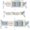
Machine learning model examples for quantum (a,b) and a hybrid (c) neural networks. For each example, the input layers have neurons equal to the feature dimensionality. (a) A one-node, multi-variational layer quantum network with strongly entangled qubits. (b) A two-quantum-node network with strongly entangled qubits. (c) A one-quantum-node, multi-variational layer hybrid network with strongly entangled qubits.

Figure A1

Example TensorFlow wrapped QNN.

Figure 1

An example classical PINN setup for the solution of an advection–diffusion equation. In this example, a and b are equation parameters, $\epsilon$ is a user-defined loss tolerance, x and t are the independent variables (network features), and the neural network solution is given by u.

Figure 4

Median and standard deviation RMSE results for the 1D spring-mass problem averaged over 10 runs for a varying number of qubits and variational layers (parameters). QPINN results are shown as black dashed lines with circles (noiseless) and dash-dotted lines with triangles (noise). The solid, gray lines with stars are the classical PINN results. All RMSEs are calculated over the physics-informed collocation points.

Figure 5

Solution convergence success rates for the $1D$ spring-mass QPINN problem with increasing qubit and variational layer counts. A successful convergence was achieved when the loss for this problem was less than $0.01$ for up to 2000 epochs. Failure occurred more often on low qubit runs.

Figure 6

The 2D Poisson quadratic manufactured solution used for QPINN solution. In this figure, the black filled circles are the physics-informed collocation points, and the x’s are boundary data for the data-driven loss contributions.

Figure 7

Single-node QPINN 10-run RMSEs at collocation points for the 2D Poisson equation with a quadratic manufactured solution for a range of qubits and nodal variational layers.

Figure 8

Mean and standard deviations of 10-run collocation point RMSEs for the 2D Poisson quadratic solution versus parameter counts for noiseless QPINNs, QPINNs with noise, and classical PINNs.

Figure 9

Noise (left) and noise-free (right) QPINN mean 10-run collocation point RMSE results for the 2D Poisson quadratic solution with increasing variational layer counts.

Figure 10

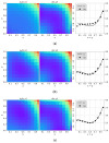
PINN (a) and QPINN (b,c) results for the 2D Poisson equation with a manufactured cubic solution. The QPINN results include device depolarizing channel noise as described in Section 3. In this figure, the left plots are the QML results, the center plots of the analytic solution for comparison, and the right $x=y$ diagonal cross sections of the analytic solution (solid black line) and QML solutions (fill circles). (a) Classical PINN results using 2 layers with 5 neurons each for a total of 51 parameters. (b) Single quantum node QPINN results comprised of 2 qubits and 4 variational layers for a total of 27 parameters. (c) Two quantum node QPINN results comprised of 2 qubits and 2 variational layers for a total of 27 parameters.

Figure 11

QPINN vs. PINN RMSEs for the Poisson equation with a cubic manufactured solution. These results include device depolarizing channel noise as described in Section 3. The QPINN results shown are for 1- and 2-quantum-node neural networks. The RMSEs calculated in this figure were calculated over 10-run solution averages at the residual collocation points.

Figure 12

Hybrid QPINN RMSEs for Burger’s equation versus the number of qubits and variational layers in the quantum network. For these results, 5 classical Keras layers preceded the quantum node. The RMSEs were calculated over the residual collocation points solutions averaged over 5 runs. In this figure, the portions of the bars below the classical PINN benchmark are colored a darker gray, while the portions above the benchmark are colored a lighter gray. Bars that fall below the benchmark RMSE are more accurate and are only colored dark gray.

Figure 13

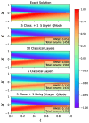
Burger’s equation exact (top plot) and predicted solutions (bottom four plots) for a series of physics-informed models. All RMSEs were calculated over the residual collocation points. In the bottom plot, noise device depolarizing channel noise as described in Section 3 has been added to the HPINN.

References

1. Kieu T. Quantum Hypercomputation. [(accessed on 5 March 2024)];Minds Mach. 2002 12:541–561. doi: 10.1023/A:1021130831101. Available online: https://api.semanticscholar.org/CorpusID:10368720. - DOI
1. D-Wave Ocean Software Documentation. [(accessed on 1 January 2024)]. Available online: https://www.dwavesys.com/solutions-and-products/ocean.
1. Aleksandrowicz G., Alexander T., Barkoutsos P., Bello L., Ben-Haim Y., Bucher D., Cabrera-Hernández F.J., Carballo-Franquis J., Chen A., Chen C. Qiskit: An Open-Source Framework for Quantum Computing. Jan, 2019. [(accessed on 13 August 2021)]. Available online: https://zenodo.org/records/2562111.
1. IBM Learning Quantum Computation Using Qiskit. [(accessed on 1 June 2021)]. Available online: http://qiskit.org/textbook.
1. Steiger D., Häner T., Troyer M. ProjectQ: An open source software framework for quantum computing. Quantum. 2018;2:49. doi: 10.22331/q-2018-01-31-49. - DOI
LinkOut - more resources