Poisson Kalman filter for disease surveillance

Abstract

An optimal filter for Poisson observations is developed as a variant of the traditional Kalman filter. Poisson distributions are characteristic of infectious diseases, which model the number of patients recorded as presenting each day to a health care system. We develop both a linear and a nonlinear (extended) filter. The methods are applied to a case study of neonatal sepsis and postinfectious hydrocephalus in Africa, using parameters estimated from publicly available data. Our approach is applicable to a broad range of disease dynamics, including both noncommunicable and the inherent nonlinearities of communicable infectious diseases and epidemics such as from COVID-19.

FIG. 1.

Diagram of the SIR model for neonatal sepsis.

FIG. 2.

(a) Summary of the inputs to the model for infant sepsis, with values used in parentheses; the remaining parameters are computed using Eqs. (20). (b) Simulation of the model for infant sepsis in Uganda assuming constant birth rate and starting from the zero initial condition $\left(S_0,I_0,R_0\right)=(0,0,0)$.

FIG. 3.

Diagram of the SIRH model for neonatal sepsis and hydrocephalus. Note that in Sec. IV we consider the linear model with $\beta =0$.

FIG. 4.

(a) Simulation of the SIRH model for Uganda starting from the zero initial condition. (b) Plot of the cumulative deaths from sepsis and hydrocephalus in the simulation. The horizontal lines are spaced so that their intersections with the curves are 365 days apart and indicate the cumulative deaths at times one year apart. The model predicts approximately 11 000 annual deaths due to sepsis and approximately 3300 annual deaths due to PIH.

FIG. 5.

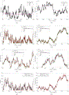
Comparison of the PKF (optimal variable gain) and the Kalman filter (optimal fixed gain) for the SIRH model with Poisson observations of the infected and hydrocephalic populations. The true (a) susceptible $S$, (b) recovered $R$, (c) infected $I$, and (d) hydrocephalic $H$ values (black) are compared to the PKF (red dashed curve) and Kalman filter (blue dotted curve) estimates. (c) and (d) also show the observations (green circles) rescaled by dividing by the constants $c_I$ and $c_H$, respectively. (e) and (f) Expanded versions of (d), enlarged to show detail. When the number of cases is large, the KF estimate of $H$ is very close to the observations, whereas the PKF adjusts to the larger observation variance and produces better estimates. Also shown are the Poisson rates (black) of (g) $I$ and (h) $H$ and the observed case numbers (red circles) from the Poisson distribution.

FIG. 6.

Comparison of the RMSE for the (a) infected and (b) hydrocephalic populations of the PKF (red solid curve, optimal variable gain) and the Kalman filter (blue solid curve, optimal fixed gain) as function of the system noise. We also compare to an oracle PKF (black dashed curve) which is given the optimal choice of $V_k=\text{diag}\left(B{\overrightarrow{x}}_k\right)$. System noise is quantified as a multiple of the base noise level $W$. The RMSE is averaged over 10⁶ filter steps.

FIG. 7.

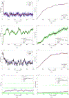
Comparison of the extended PKF (optimal variable gain) and the extended Kalman filter (optimal fixed gain for the noncontagious equilibrium) for the contagious SIRH model with Poisson observations of the infected and hydrocephalic populations. We compare the true $S$, $I$, $R$, and $H$ values (black solid curve) to the PKF (red dashed curve) and Kalman filter (blue dotted curve) estimates. We show (a)–(d) a standard observation rate $c_I=0.2/T_S$ and $c_H=0.6/T_R$ and (e)–(h) a low observation rate $c_I=0.0002/T_S$ and $c_H=0.0006/T_R$. The infected and hydrocephalic plots also show the observations (green circles) rescaled by dividing by the constants $c_I$ and $c_H$, respectively. The system is initialized at the noncontagious equilibrium and run forward with $\beta ={10}^{-6}$ simulating the introduction of a contagious source of infection which moves the system to a new equilibrium.

FIG. 8.

(a) and (b) Comparison of the RMSE of the EPKF (red solid curve, optimal variable gain) and the EKF (blue solid curve, optimal fixed gain) as a function of the system noise. We also compare to an oracle EPKF (black dashed curve) which is given the optimal choice of $V_k=\text{diag}\left(B{\overrightarrow{x}}_k\right)$. System noise is quantified as a multiple of the base noise level $W$. The RMSE is averaged over 10⁶ filter steps. The two-standard-deviation regions around the EPKF and EKF estimates are shown using the variance estimated by the respective filters for (c) the standard observation rate and (d) the low rate from Fig. 7.

References

1. Zaman G, Kang YH, and Jung IH, Proc. KSIAM 3, 31 (2007).
1. Yusuf TT and Benyah F, World J. Model. Simul 8, 194 (2012).
1. Zaman G, Kang YH, and Jung IH, BioSystems 93, 240 (2008). - PubMed
1. Sharomi O and Malik T, Ann. Oper. Res 251, 55 (2017).
1. Di Giamberardino P and Iacoviello D, Proceedings of the 2019 23rd International Conference on System Theory, Control and Computing (ICSTCC) (IEEE, Piscataway, 2019), pp. 733–738.
LinkOut - more resources