Perpetual step-like restructuring of hippocampal circuit dynamics

Abstract

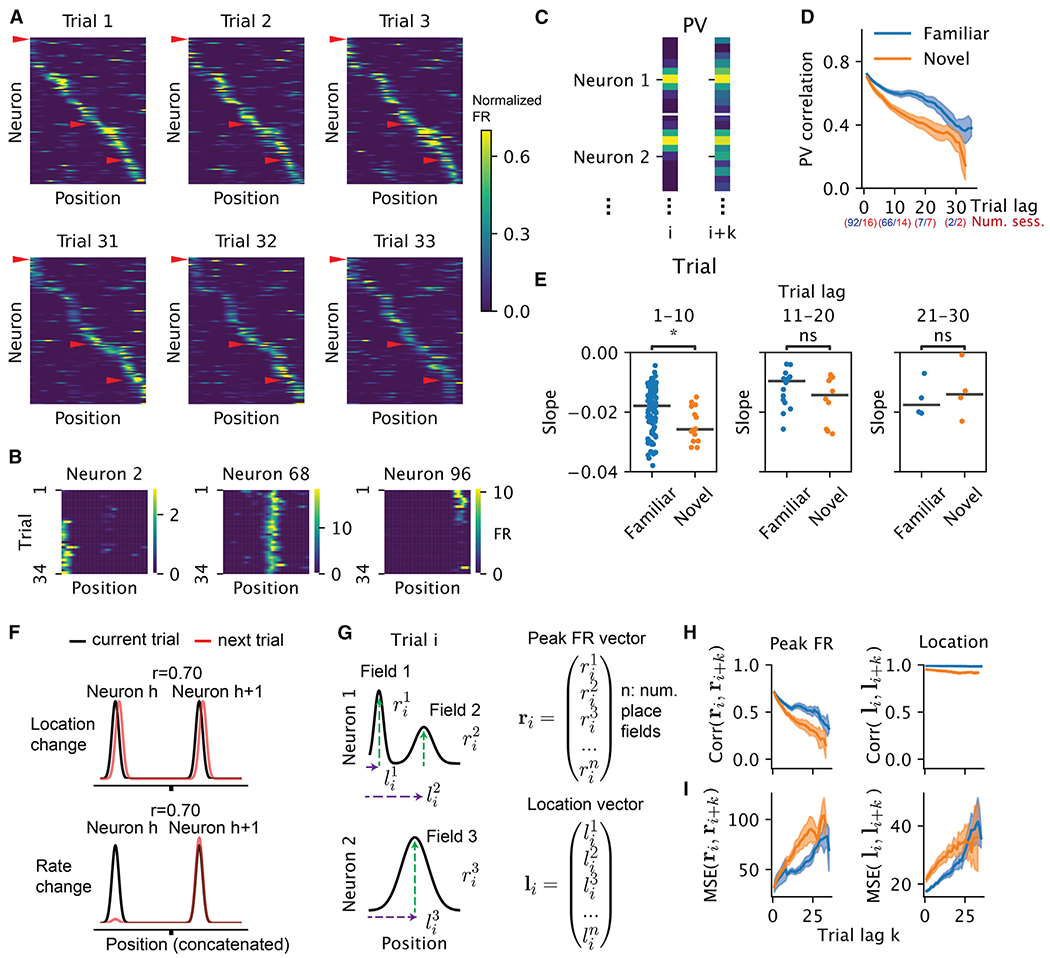
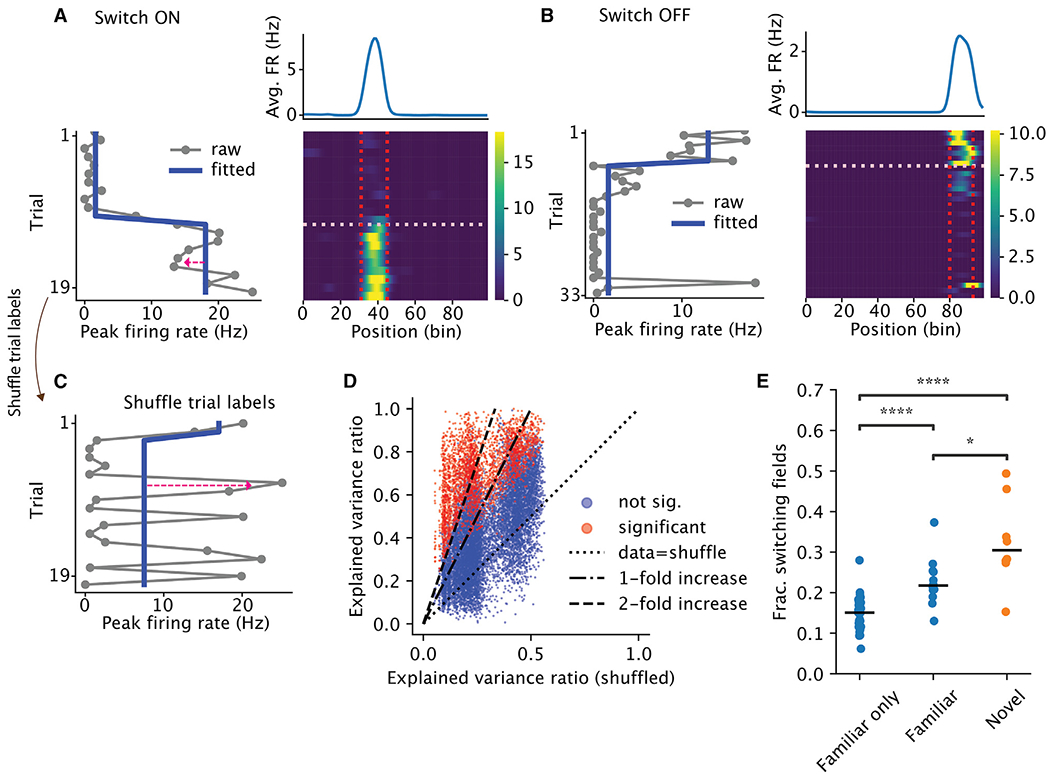
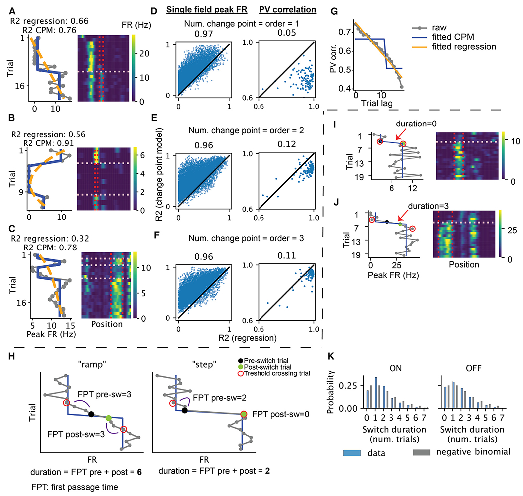
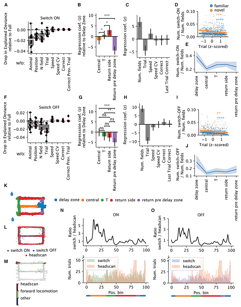
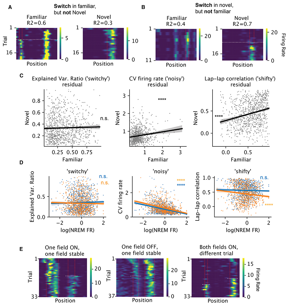
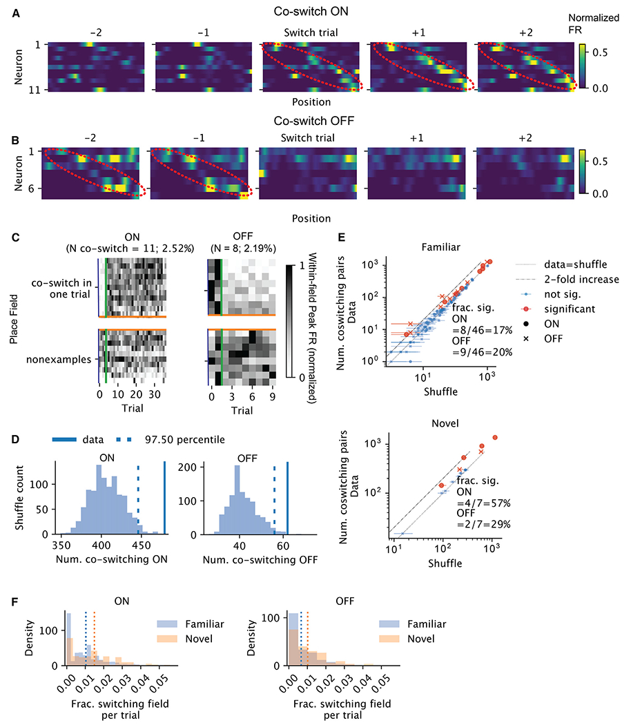
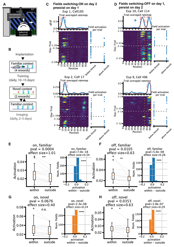
Representation of the environment by hippocampal populations is known to drift even within a familiar environment, which could reflect gradual changes in single-cell activity or result from averaging across discrete switches of single neurons. Disambiguating these possibilities is crucial, as they each imply distinct mechanisms. Leveraging change point detection and model comparison, we find that CA1 population vectors decorrelate gradually within a session. In contrast, individual neurons exhibit predominantly step-like emergence and disappearance of place fields or sustained changes in within-field firing. The changes are not restricted to particular parts of the maze or trials and do not require apparent behavioral changes. The same place fields emerge, disappear, and reappear across days, suggesting that the hippocampus reuses pre-existing assemblies, rather than forming new fields de novo. Our results suggest an internally driven perpetual step-like reorganization of the neuronal assemblies.

Keywords: CP: Neuroscience; change point detection; place fields; plasticity; pre-existing assemblies; quantal change; remapping; representational drift.

Figure 1.. Stability and change of single units and population activity

(A) Population rate maps of hippocampal place cells during early and late trials. Place cells were sorted by the peak of the place fields on trial 1. (When there were multiple fields, we used the fields with the largest within-field peak firing rates. Only place cells with spatial information larger than 1 bit/spike are displayed here for ease of visualization; n = 114 of 264 place cells for one direction of turn in the figure-8 maze.) Color represents normalized firing rate. (B) Rate maps of three example neurons, marked by red arrowheads in (A), showing place field emergence (left), stable firing (middle), and place field disappearance (right). (C) Schematic for constructing the population vectors (PVs) in (D). The rate maps for all neurons were concatenated on a given trial to form a PV. The Pearson correlation between PVs from a pair of trials was computed. All trial pairs with lag k were averaged to produce the mean PV correlation per trial lag. (D) Population rate map correlations as a function of trial lag (only place cells are included). Blue and orange correspond to familiar and novel sessions, respectively. Shaded area corresponds to 95% confidence interval, where each data point is the correlation between two trials within one session. The numbers of included sessions for blocks of trials are indicated in parentheses. (E) Comparing the slope of PV correlation decay between familiar and novel environments in three ranges of trial lags. Trial lag 1–10, n = 106, Wilcoxon rank-sum test, p = 0.02, Cohen’s d = 0.58; trial lag 11–20, n = 26, p = 0.3, Cohen’s d = 0.54; trial lag 21–30, n = 8, p = 0.68, Cohen’s d = −0.35. Asterisks indicate the significance level for all figures (*0.01 < p ≤ 0.05; **0.001 < p ≤ 0.01, ***0.0001 < p ≤ 0.001; ****p ≤ 0.0001). We note that the lack of significance could be due to fewer sessions present at the later ranges. (F) Schematics of different hypothetical mechanisms inducing a population-level decorrelation. Each Gaussian bump represents the tuning curve of one place cell. The Pearson correlation r is taken between the black (current trial) and red (next trial) curves. (G) Schematics for how the within-field peak firing-rate vector and place field location vector were constructed in (H) and (I). (H) Correlation of within-field peak population firing rate (left) and peak location (right) of place cells as a function of trial lag. (I) Similar to (H), but instead of correlation, the normalized squared Euclidean distance (equivalent to mean squared error, MSE) is shown as a function of trial lags.

Figure 2.. Place cells exhibit discrete switching of firing rate

(A and B) Examples of place cells with place fields that switched ON (A) or OFF (B). Bottom right is the rate map, i.e., firing rate (color) as a function of position (x axis) and trial (y axis). Vertical lines mark the boundary of the place fields. The horizontal line marks the switch trial. Bottom left is the peak within-field firing rate across trials. The red arrow in (A) highlights the reconstruction error. The blue line is the fitted step function. Top right is the trial-averaged rate map. (C) Peak within-field firing rate from (A), with the trial label shuffled. (D) Explained variance ratio from the best change-point model, data vs. shuffle. Each dot is a place field, colored by whether the field had significant switching. (E) Each dot is the fraction of switching fields from one session, grouped by whether the session came from an animal that experienced only the familiar environment (“Familiar only,” n = 34, median = 0.15), the session was a familiar-environment session but came from an animal that also experienced the novel environment on that day (“Familiar,” n = 12, median = 0.22), or the session was a novel environment (“Novel,” n = 8, median = 0.3). Horizontal bars are the medians. Two-sided Wilcoxon rank-sum test: Familiar only vs. Familiar, p = 4 × 10⁻⁵; Familiar vs. Novel, p = 0.01; Familiar only vs. Novel, p = 1.7 × 10⁻⁵.

Figure 3.. Discrete and continuous models of the trial-to-trial changes of within-field firing rates and population vectors

(A–C) Example neurons illustrate the comparison between change-point model and a continuous polynomial regression model. Left: gray, within-field peak firing rate as a function of trial; blue, fitted change-point model (i.e., a step function); orange, fitted polynomial regression. Right: rate maps of the selected neuron. The vertical lines mark the boundary of the place field, while the horizontal lines mark the detected change points. Neurons A, B, and C have one, two, and three change points/polynomial order, respectively. (D–F) Explained variance ratio of the change-point model vs. that of the polynomial regression for each place field (left) and the population vector from each session (right, different turns of the T maze and different directions of the linear maze were treated separately). For individual place fields, the models are fitted to the within-field firing rate across trials. For population vectors, the models are fitted to predict population vector correlation (averaged across trial pairs) using trial lag. (G) Example of the comparison between a discrete change-point model and a continuous polynomial regression model (CPM) for the population vector correlation as a function of trial lag. (H) Schematics demonstrating the differences in first passage time (FPT) of threshold crossing in data better characterized as a “ramp” (left) vs. a “step” (right). Threshold crossing is defined as above the predicted firing rate by the step model post-switch-ON and below the predicted pre-switch-ON firing rate and vice versa for OFF. Post-switch trial is the change point given by the change point detection, and pre-switch trial is one trial before. (I and J) Examples demonstrating switching with different switch durations, measured by the number of trials between the first pre-switch and the post-switch threshold crossing trial (red circle) minus one. (K) Distributions of the switch durations for switch-ON and -OFF (blue), compared with a negative binomial (p = 0.5) with two successes (gray).

Figure 4.. Spatial-temporal and behavioral modulation of switching

(A–C) Poisson generalized linear model (GLM) predicting the number of switch-ON occurrences per arm and trial within one session (n = 5,131 arms × trials from 46 sessions from 11 animals). (A) Drop in explained deviance relative to the full model when one predictor is removed in the GLM. Each dot is one random split in the 5-fold cross-validation. (B) Spatial regression coefficients, in standardized units: each variable represents the gain in the probability of switching when the animal is in one arm relative to the delay zone. Error bars reflect 95% confidence intervals (CIs), based on asymptotic standard errors from the Fisher information matrix. (C) The rest of the regression coefficients. (D) The number of switch-ON occurrences normalized by the number of fields as a function of trial (Z scored within each session for comparison across sessions with different numbers of trials). Blue, familiar; orange, novel (familiar: n = 1,029 trials, Pearson r = −0.15, p = 1.3 × 10⁻⁶; novel: n = 281 trials; Pearson correlation r = −0.23, p = 1.3 × 10⁻⁴). (E) The number of switch-ON occurrences normalized by the number of fields as a function of the arms. Each data point is one session. Shaded region reflects the 95% CI. (F–J) Similar to (A)–(E), but for switching OFF occurrences. (I) Familiar: Pearson r = −0.2, p = 3.3 × 10⁻¹¹; novel: Pearson r = −0.18, p = 2.7 × 10⁻³). (K) Schematic of the maze, with each arm colored differently. (L) Detected head-scanning events projected onto the maze. (M) Distribution of the head scans and switches on the maze for one example session. (N and O) Top: the ratio as a function of position between the number of trials when switch-ON (N)/-OFF (O) occurs and the number of trials when head scans occur. Bottom: the number of trials when switches (green or purple)/head scans (pink) occur as a function of position.

Figure 5.. Switching is not a single-neuron property

(A) Example neuron with no switch-ON field in the familiar and with switch-ON field in the novel maze. R2: explained variance ratio of the one-change-point model. Vertical lines mark the field boundary and the horizontal line marks the switch trial. (B) Example neuron with switch-ON field in the familiar but no switch-ON field in the novel maze. (C) For each neuron (per dot, n = 955), the relationship between familiar and novel maze for each metric of variability (per column) is shown, after regressing out the effect of firing rate during NREM sleep. The firing rates were first log-transformed. The residuals are significantly correlated across environments for CV of within-field peak firing rate (left, standardized linear regression coefficients t = 4.8, R2 = 0.02, p < 10⁻⁵) and lap-lap rate map correlation (middle, t = 7.9, R2 = 0.06; p < 10⁻¹⁴), but not for the explained variance ratio from the change-point model (right, t = 0.9, R2 = 0.0008, p = 0.37). The error bands show 95% CI for the regressions. (D) For each neuron (per dot), the relationship between each metric of variability (per column) and its log-firing rate during NREM sleep. Blue and orange: familiar and novel environments, respectively. (Standardized linear regression coefficients and p values: noisy: familiar, t = −11.1, p = 3.6 × 10⁻²⁷; novel, t = −12.6, p = 1.5 × 10⁻³³; shifty: familiar, t = −0.8, p = 0.4; novel, t = −3.6, p = 0.000326; switchy: familiar, t = 0.9, p = 0.4; novel, t = −0.6, p = 0.5). (E) Examples of subfields of a neuron showing different switching behavior.

Figure 6.. Network coordination of switching

(A) Activities of example neurons whose fields co-switched ON in the vicinity of the co-switching trial. Each heatmap is the rate map for different neurons (row) for one trial. The rows are sorted by the locations of the place fields that switched together. The color reflects the normalized firing rate. The x axis is position. The emerging sequence is highlighted in red ellipsoids. (B) Similar to (A), but for fields that switched OFF together. The fading sequence is highlighted in red ellipsoids. (C) Within-field peak firing rates per field across trials (normalized across all trials), for the same set of neurons as in (A). Each row is a field. Above the orange lines are the fields that co-switched ON at the trial marked by the green vertical lines, whereas below are the randomly selected fields that did not switch ON that trial. Left contains the fields of the neurons shown in (A) and right contains the fields of the neurons shown in (B). (D) Shuffle test result for the number of pairs of fields that co-switched ON on some trials, for the sessions in (A) (left) and (B) (right). (E) For each session, the number of co-switching pairs vs. shuffle median. The error bars mark the 95% CI from shuffle tests. Red dots are sessions with significant co-switching of neurons. Circles and crosses correspond to co-switching ON and cross OFF fields, respectively. Top, familiar, and bottom, for novel context. (F) Histograms of the fraction of switching fields for ON (left) and OFF (right) in each trial (excluding the first and last two trials). Blue is familiar and orange is novel context. Vertical lines mark the means.

Figure 7.. Switching is biased by pre-existing fields

(A) Experimental setup of the imaging experiment. (B) Behavior timeline. (C and D) Example neurons that had a place field that switched ON on day 2 (C) or was OFF on day 1 (D). Top: trial-averaged rate map in blue, with field mask in dotted red line. Bottom left: rate map; red vertical lines mark the boundary of the fields, while orange vertical lines mark the “outside” region for the quantifications in (E)–(H). White horizontal line marks the change in the day. Bottom right: binary variable of whether the within-field activation is above the place field detection threshold at each trial. Arrow in (D) (top) marks the place field of interest among the two fields. Note: (D) (bottom) is an example for both scenarios in (C) and (D). (E–H) Quantifications of within- vs. outside-of-field activation (n = 14). For fields that switch ON (E and G) on the second day, the quantification is done on the first day using the field detected on the second day. The opposite is true for fields that switch OFF (F and H), i.e., detected on the first day and quantified on the second day. Left: median dF/F across trials, averaged across all fields within one session, separated into within vs. outside of the place fields. Right: histogram of within minus outside-of-field dF/F of all fields pooled across sessions. Wilcoxon rank-sum tests and Cohen’s d are used for significance test and effect size.

References

1. O’Keefe J, and Nadel L (1978). The Hippocampus as a Cognitive Map (Clarendon Press; ).
1. Thompson LT, and Best PJ (1990). Long-term stability of the place-field activity of single units recorded from the dorsal hippocampus of freely behaving rats. Brain Res. 509, 299–308. 10.1016/0006-8993(90)90555-. - DOI - PubMed
1. Manns JR, Howard MW, and Eichenbaum H (2007). Gradual Changes in Hippocampal Activity Support Remembering the Order of Events. Neuron 56, 530–540. 10.1016/j.neuron.2007.08.017. - DOI - PMC - PubMed
1. Ziv Y, Burns LD, Cocker ED, Hamel EO, Ghosh KK, Kitch LJ, El Gamal A, and Schnitzer MJ (2013). Long-term dynamics of CA1 hippocampal place codes. Nat. Neurosci 16, 264–266. 10.1038/nn.3329. - DOI - PMC - PubMed
1. Sheintuch L, Geva N, Baumer H, Rechavi Y, Rubin A, and Ziv Y (2020). Multiple Maps of the Same Spatial Context Can Stably Coexist in the Mouse Hippocampus. Curr. Biol 30, 1467–1476.e6. 10.1016/j.cub.2020.02.018. - DOI - PubMed
LinkOut - more resources