Advanced Methods for Analyzing in-Situ Observations of Magnetic Reconnection

Abstract

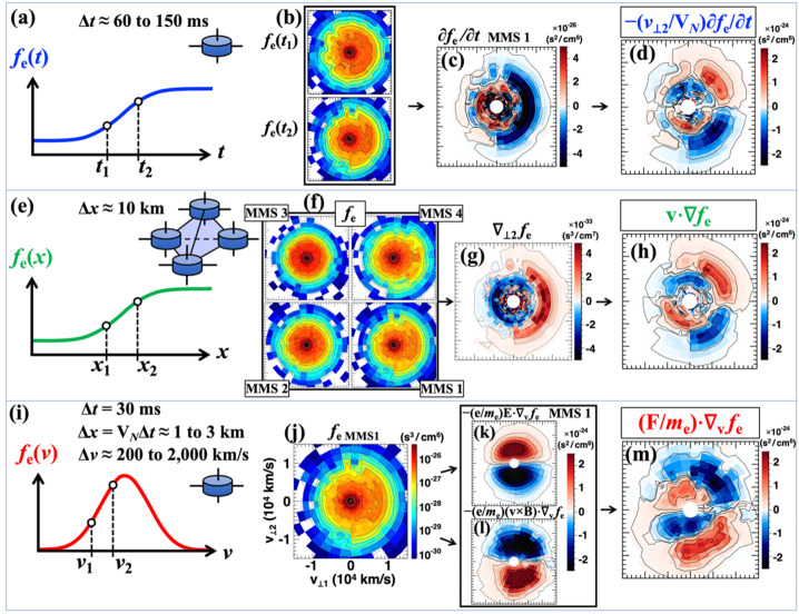
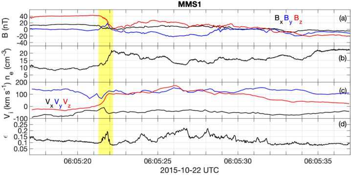
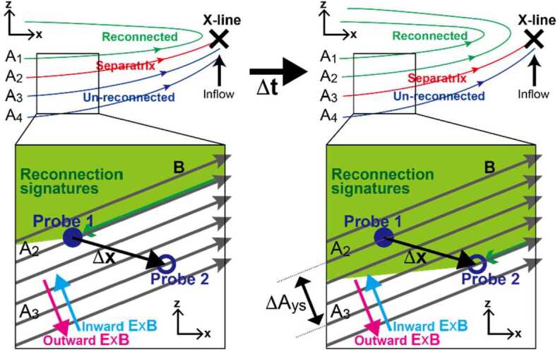
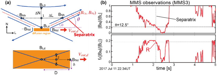
There is ample evidence for magnetic reconnection in the solar system, but it is a nontrivial task to visualize, to determine the proper approaches and frames to study, and in turn to elucidate the physical processes at work in reconnection regions from in-situ measurements of plasma particles and electromagnetic fields. Here an overview is given of a variety of single- and multi-spacecraft data analysis techniques that are key to revealing the context of in-situ observations of magnetic reconnection in space and for detecting and analyzing the diffusion regions where ions and/or electrons are demagnetized. We focus on recent advances in the era of the Magnetospheric Multiscale mission, which has made electron-scale, multi-point measurements of magnetic reconnection in and around Earth's magnetosphere.

Keywords: Data analysis techniques; Electron diffusion region; In-situ measurements; Magnetic reconnection; Magnetosphere.

Fig. 1

Typical geometry (magnetic field and plasma inflow and outflow pattern) of (a) magnetotail (approximately antiparallel and symmetric) reconnection and (b) magnetopause (normally guide-field and asymmetric) reconnection. Note that the reconnection electric field $E_{\mathrm{r}}$ in LMN coordinates typically has a different polarity for the two cases

Fig. 2

Schematic of the northern cusp region with the Polar satellite simultaneously observing incident ions on newly opened magnetic field lines which originate at the magnetopause reconnection location and mirrored ions returning from the ionosphere. The color distribution function shows the cutoff velocities $V_{\mathrm{e}}$ and $V_{\mathrm{m}}$ of the incident and mirrored ion beams, respectively

Fig. 3

The distance to the magnetopause reconnection site from the cusp position of the Polar satellite on 11 April 1996 (top panel). The location of the magnetopause reconnection site as seen from dawn (bottom left panel). The magnetopause magnetic shear angle with the reconnection site location (black squares) as seen from the Sun for the 11 April 1996 Polar cusp crossing (bottom right panel)

Fig. 4

Evolution of the magnetic field line topology and spacecraft locations for an MMS dayside magnetopause reconnection event on 24 December 2016. Field lines are traced from MMS and from Geotail, and from other start locations. At time 14:54 UT, MMS was predicted by the SWMF model to be near the X-line, and on open field lines (green) connected to the southern cusp. Then the IMF $B_y$ changed sign, and at 15:20:30 UT, both MMS and Geotail were predicted to be on open field lines (green) connected to the northern polar cap, and their mapped field lines passed less than a half R_E (R_E: Earth radius) apart at the magnetopause. About a minute after the predicted connection, Geotail started observing O+ presumably from the magnetosphere, evidence of that connection

Fig. 5

The kNN DM method outline (Sitnov et al. 2021): ($\mathbf{a}$) selecting nearest neighbors for the event of interest (blue circle) in the 5D global parameter state-space; ($\mathbf{b}$) finding the corresponding subset in the magnetic field database (gray dots overplotted on the color-coded equatorial $B_z$ distribution) and using it to fit the magnetic field model and to yield 2D magnetic field distributions (here the equatorial slice) as well as ($\mathbf{c}$) 3D magnetic field distributions. The example shown here is for the 11 July 2017 MMS EDR event Torbert et al. 2018) with the color-coded equatorial $B_z$ (in nT, saturated at 5 nT for better visualization) and a few sample field lines. Panels ($\mathbf{a}$) and ($\mathbf{b}$) are adapted from Sitnov et al. (2019)

Fig. 6

From left to right: representation of the magnetic field lines in the XY (left), YZ (middle) planes and in 3D (right) as predicted by the KF94 magnetostatic model (top panels) or reconstructed from in situ data (bottom panels). On the four leftmost panels, the color codes the value of the $B_x$ component of the magnetic field. Coordinates are from the SWI system

Fig. 7

STD analysis for the 16 Oct 2015 magnetopause reconnection event. ($\mathbf{a}$) MDD eigenvalues, (b–d) STD structure velocity components in the local MDD gradient directions, ${\hat{\mathbf{e}}}_l$, ${\hat{\mathbf{e}}}_m$, and ${\hat{\mathbf{e}}}_n$ respectively, ($\mathbf{e}$) magnetic field averaged over the four MMS spacecraft, (f–h) STD structure velocity in the fixed LMN coordinates. The dotted curves are the instantaneous velocities, and the solid curves are smoothed over a time scale of 0.5 s

Fig. 8

A reconstruction of the magnetic field lines as MMS approached an electron diffusion region at 13:07:02.25 UT on 16 October 2015. The four MMS spacecraft locations are colored diamonds: (black, red, green, blue) are the standard colors for (MMS1, 2, 3, 4) respectively. The colored arrows show the projection of the electron flow velocity into this $LN$ plane. The purple arrows at each spacecraft show the direction of the field and the lengths the relative magnitude of the magnetic field at that location

Fig. 9

Reduced quadratic reconstruction for 16 October 2015, 13:07:02.25 UT. The black, red, green, and blue spheres and curves show the positions and magnetic field lines passing through MMS1, 2, 3, and 4, respectively. The gold curves are other magnetic field lines with the cones indicating the direction and magnitude

Fig. 10

($\mathbf{a}$) Relative differences (${\gamma }_B,{\gamma }_j$) and ($\mathbf{b}$) quality indicators ($Q_{\mathrm{model}},Q_{curl}$) for a sensitivity run with weighting factors $w_B$ and $w_C$ both set to 0. The very small relative difference values (≪1) highlights that the empirical model results in a very good fit between the modeled and measured fields at the prescribed spatial points

Fig. 11

The left column shows fields measured by MMS constructed into a 2D map based on the spacecraft trajectory. The middle column shows PIC simulation data in the same region of the reconnection geometry for comparison, while the right column shows the simulation data plotted over the entire domain. Adapted from Schroeder et al. (2022)

Fig. 12

2D maps of the magnetic field ($\mathbf{a}$) and electron streamlines ($\mathbf{b}$) from the EMHD reconstruction applied to data from the magnetotail EDR encounter by MMS3 on 11 July 2017. The arrows show the projection onto the reconstruction plane of the measured magnetic fields ($\mathbf{a}$) and electron velocities in the structure-rest frame ($\mathbf{b}$). The axial current density ($\mathbf{a}$) and axial magnetic field component ($\mathbf{b}$) are shown in color. The blue and red bars in Fig. 12 are the projection of the GSM $x$ and $z$ axes, respectively. Adapted from Hasegawa et al. (2021)

Fig. 13

Magnetospheric Multiscale (MMS) spacecraft 3 observations of an electron diffusion region at 2233:50-2234:15 UT on 11 July 2017. The top panel shows the three components and the strength of the magnetic field in geocentric solar ecliptic (GSE) coordinates ($B_x$, blue; $B_y$, green; $B_z$, red; and $\left|\mathbf{B}\right|$, black). The second panel shows the components of the electron velocity in the same color scheme. The final panel shows $\sqrt{Q_e}$

Fig. 14

MMS data in the magnetopause reconnection event on 16 October 2015. The X-line crossing was around 13:07:02.4 UTC. From top the plotted quantities are the magnetic field in GSE coordinates ($\mathbf{B}$_GSE), the Zenitani measure ($\mathbf{j}\mathbf{\cdot }{\mathbf{E}}^{\prime }$) and pressure-strain rate ($-(\mathbf{P}\mathbf{\cdot }\mathrm{\nabla })\mathbf{\cdot }\mathbf{u}$), electron ($-({\mathbf{P}}_{\mathrm{e}}\mathbf{\cdot }\mathrm{\nabla })\mathbf{\cdot }{\mathbf{u}}_{\mathrm{e}}$) and ion ($-({\mathbf{P}}_{\mathrm{i}}\mathbf{\cdot }\mathrm{\nabla })\mathbf{\cdot }{\mathbf{u}}_{\mathrm{i}}$) pressure-strain rates, compressive ($-p^{\left(e\right)}{\theta }^{\left(e\right)}$) and incompressive ($-{\mathrm{\Pi }}_{ij}^{\left(e\right)}{D}_{ij}^{\left(e\right)}$) pressure-strain rates for electrons, and compressive ($-p^{\left(i\right)}{\theta }^{\left(i\right)}$) and incompressive ($-{\mathrm{\Pi }}_{ij}^{\left(i\right)}{D}_{ij}^{\left(i\right)}$) pressure-strain rates for ions

Fig. 15

MMS observation of a magnetotail current sheet crossing along the trajectory shown in white in panel ($\mathbf{e}$). ($\mathbf{a}$) The tetrahedral-averaged magnetic field, ($\mathbf{b}$) current density calculated from the curlometer technique, ($\mathbf{c}$, $\mathbf{d}$) electron vorticity and its magnitude compared to $\omega$_ce. Panel ($\mathbf{f}$) illustrates the origin of the enhanced electron vorticity near the northern/southern edge of the EDR. Adapted from Hwang et al. (2019)

Fig. 16

MMS observations of the Eriksson et al. event (adapted from Qi et al. 2022). ($\mathbf{a}$) Magnetic field and ($\mathbf{b}$) electric field averaged over four spacecraft. ($\mathbf{c}$) Radius of curvature $R_{\mathrm{c}}$ normalized to the electron (red) and ion (blue) gyro-radius. ($\mathbf{d}$) Electron bulk flow velocity and ($\mathbf{e}$) MFT velocity ${\mathbf{U}}_{\psi }$, where the ion bulk flow velocity is subtracted. Dotted lines denote the upstream Alfvén speed. ($\mathbf{f}$) $\mathrm{\nabla }\cdot {\mathbf{U}}_{\psi }$ normalized to $f_{\mathrm{ce}}$. ($\mathbf{g}$) Sketch of the trajectory of MMS and expected MFT inflows and outflow, adapted from Eriksson et al. (2018)

Fig. 17

EDR event from Burch et al. (2016a) with detected crescent distribution functions. The top four panels show MMS2 observations of the magnetic field $\mathbf{B}$, electron-frame electric field ${\mathbf{E}}^{\prime }$ (showing the departure from the ideal conditions), electron and ion densities, and the energy conversion rate $\mathbf{j}\mathbf{\cdot }{\mathbf{E}}^{\prime }$. Four of the identified “crescents” are shown below the time series plots, both in classical phase space density units (top) and in transformed 32×32 images (bottom). The two-dimensional electron distribution slices are displayed in the $v_{\mathrm{\perp }1}$-$v_{\mathrm{\perp }2}$ plane where $v_{\mathrm{\perp }1}$ is directed along ($-{\mathbf{u}}_{\mathrm{e}}\times \mathbf{B})\times \mathbf{B}$ (approximately the $\mathbf{E}\times \mathbf{B}$ direction, where $\mathbf{E}$ is the electric field, and ${\mathbf{u}}_{\mathrm{e}}$ is the electron bulk velocity), and $v_{\mathrm{\perp }2}$ is directed along $-{\mathbf{u}}_{\mathrm{e}}\times \mathbf{B}$ (approximately the direction of $\mathbf{E}$)

Fig. 18

Example of the calculation of the $M$ component of the anomalous resistivity $\mathbf{D}$. ($\mathbf{a}$) Background (lowpass filtered) components of the electron number density $n$ (MMS1-MMS4 data are plotted in black, red, green, and blue, respectively) and $\langle n\rangle$ calculated by averaging over the four spacecraft (magenta line). ($\mathbf{b}$) and ($\mathbf{c}$) $\delta$$E_M$ and $\delta$$n$ for the four spacecraft. ($\mathbf{d}$) $\delta$$n$$\delta$$E_M$ calculated for the four spacecraft, and the four-spacecraft averaged $\delta$$n$$\delta$$E_M$ (cyan), and 〈$\delta$$n$$\delta$$E_M\rangle$ (magenta) obtained by low-pass filtering the averaged $\delta$$n$$\delta$$E_M$. I $M$ component of $\mathbf{D}$ calculated from 〈$\delta$$n$$\delta$$E_M\rangle$ and $\langle n\rangle$. In all panels ($\mathbf{a}$)-($\mathbf{d}$) the quantities from MMS2-MMS4 have been time shifted so they cross the current sheet at the same time

Fig. 19

This figure presents a visual summary of the velocity-space structure and qualitative balance of the three Vlasov equation terms for an electron-scale current sheet. The computation technique for (a-d) $\partial f_{\mathrm{e}}$/$\partial t$, (e-h) $\mathbf{v}\cdot \mathrm{\nabla }{f}_{\mathrm{e}}$, and (i-m) ($\mathbf{F}/m_{\mathrm{e}}$)$\cdot {\mathrm{\nabla }}_{\mathbf{v}}{f}_{\mathrm{e}}$ is shown schematically. Each velocity-space panel represents a slice taken in the $v$_⊥1-$v$_⊥2 plane. In this example, ${\hat{\mathbf{e}}}_N$ points roughly along ${\hat{\mathbf{e}}}_{\mathrm{\perp }2}$, so that the quantities shown in panels (d) and (h) are roughly equivalent. Comparing panels (h) and (m), one can see a notable quadrupolar pattern but with a polarity difference, suggesting that Eq. (47) is roughly satisfied in velocity space under the assumption of negligible $\partial f_{\mathrm{e}}$/$\partial t$ (panel (c)). Adapted from Shuster et al. (2023)

Fig. 20

Example of electron non-Maxwellianity for the electron diffusion region crossing observed by MMS1 on 22 October 2015. ($\mathbf{a}$) Magnetic field. ($\mathbf{b}$) electron number density. ($\mathbf{c}$) Ion bulk velocity. ($\mathbf{d}$) Non-Maxwellianity $\epsilon$ of electrons. The EDR is indicated by the yellow-shaded region

Fig. 21

MMS and PIC simulation comparisons of non-Maxwellianity in a magnetotail electron diffusion region. ($\mathbf{a}$) The 2D profile of non-Maxwellianity surrounding the EDR with the MMS trajectory shown (dotted magenta line). Different electron non-Maxwellianity quantities as observed ($\mathbf{b}$,$\mathbf{c}$) by MMS and ($\mathbf{d}$,$\mathbf{e}$) in PIC, where ${\bar{M}}_{KP}$ (Eq. (59)) is computed using $s$ (blue) and $s_V$ (Eq. 61) (green). The MMS panels show a larger view than is depicted in the simulation for comparison with other published studies. Vertical dashed lines (and the “x” in panel $\mathbf{a}$) indicate where electron distributions were obtained ($\mathbf{f}$,$\mathbf{g}$,$\mathbf{h}$) by MMS and ($\mathbf{k}$) in PIC simulation. PIC distributions in ($\mathbf{i}$,$\mathbf{j}$) were taken outside of the bounds of panel ($\mathbf{a}$) from locations representative of the regions MMS sampled. Adapted from Argall et al. (Phys. Plasmas, 29, 022902, 2022; licensed under a Creative Commons Attribution (CC BY) license)

Fig. 22

MMS data in the event on 11 July 2017. ($\mathbf{a}$) MMS data for the field quantities and the distance $N$ from the neutral line. ($\mathbf{b}$) Electron VDF at the neutral line. ($\mathbf{c}$) VDF at $t$=$t_1$. ($\mathbf{d}$) Comparison between the theory (blue, red, green curves by Eq. (65)) and the multi-crescent VDF. Adapted from Bessho et al. (2018)

Fig. 23

Schematic of a reconnecting current sheet in motion in the $x$-$z$ plane during $\mathrm{\Delta }t$, focusing on a region near the separatrix boundary where two probes separated by $\mathrm{\Delta }\mathbf{x}$ sequentially detect the separatrix signatures (adapted from Nakamura et al. 2018a). The field line motion (E×B drift velocity) can be inward (cyan arrow) or outward (magenta arrow), depending on the magnitude of the reconnection electric field and the magnitude and direction of the structure velocity

Fig. 24

($\mathbf{a}$) Sketch of the reconnection geometry around the diffusion region (adapted from Liu et al. 2017). ($\mathbf{b}$) MMS observations of $\left|B_N\right|/\left|B_L\right|$ and $f_{\mathrm{r}}$ (Eq. (69)) during the separatrix crossing on 11 July 2017 (adapted from Nakamura et al. 2018b)

Fig. 25

Burst memory buffers at risk of being overwritten. ($\mathbf{a}$) Amount of Category 0 (purple), 1 (red), 2 (yellow), 3 (green), and 4 (blue) stored or HELD onboard MMS, shown in terms of the number of burst buffers (left axis) and the corresponding hours of data (right axis). ($\mathbf{b}$) The amount of overwritten data in terms of Category (color), memory buffers (left axis) and total time (right axis). Category 0 data are for special operations (e.g., calibration) or critical science data; selections are rare and are transmitted to ground as soon as the downlink is available, so no Category 0 buffers are present in the figure

Fig. 26

Data that the SITL uses to make selections. The SITL views data from the regions of interest, ROI 1, 2, and 3, as it becomes available, and uses a tool to interact with the plot, make selections, and submit them to the science data center. Quantities and scales are purposefully not shown except for the ABS (second to last panel) and SITL (last panel) selections. Note that while the SITL basically selected the same intervals (vertical bars) as the ABS, the SITL selected many more

Fig. 27

The GLS and ABS are complementary systems that make selections of high interest to the SITL. (a) Comparison of all selections; the SITL selects a significant number of selections made by both the GLS (71%) and ABS (64%). (b) Comparison of selections designated as magnetopause (MP) crossings by the SITL. In both cases, there is little overlap between the GLS and ABS. Adapted from Argall et al. (2020)

Fig. 28

MMS observations on 31 December 2015 (adapted from Nguyen et al. 2022a). The top to fourth panels show the ion density, magnetic field, ion velocity in GSM coordinates, and omnidirectional differential energy fluxes of ions. The bottom panel shows the evolution of the label (blue), intentionally shifted for visual inspection, and the prediction made by the ML algorithm (black), in which “0” means the magnetosphere, “1” the magnetosheath, and “2” the solar wind

Fig. 29

Example of plasma region classification of MMS data on 16 October 2015. The panels from top to bottom show ($\mathbf{a}$) the magnetic field, ($\mathbf{b}$) plasma density, ($\mathbf{c}$) ion velocity, ($\mathbf{d}$) ion energy spectrum, and ($\mathbf{e}$) the probabilities provided by the classifier

Fig. 30

The four FPI electrostatic deflection states (top four images), each composed of a full 32-step energy sweep and obtained at 7.5 ms cadence for electrons, are combined to produce a full Level 2 “skymap” (bottom left images) every 30 ms (adapted from Rager et al. 2018)

Fig. 31

The spline interpolation technique does an excellent job of recovering electron bulk velocity at 7.5 ms resolution (green line) (adapted from Rager et al. 2018). The top three panels show three components of the electron convective electric field at 30 ms (red) and 7.5 ms (green) resolutions. The perpendicular electric field measured by the double probe instruments (Ergun et al. ; Lindqvist et al. 2016), averaged down to 7.5 ms, is shown in black. The bottom two panels show the electron pressures in the directions parallel and perpendicular to the magnetic field

References

1. Andreeva VA, Tsyganenko NA (2016) J Geophys Res Space Phys 121:2249–2263. 10.1002/2015JA022242
1. Argall MR, Small CR, Piatt S, et al. (2020) Front Astron Space Sci 7:54. 10.3389/fspas.2020.00054 - PMC - PubMed
1. Argall MR, Barbhuiya MH, Cassak PA, et al. (2022) Phys Plasmas 29:022902. 10.1063/5.0073248
1. Aunai N, Hesse M, Kuznetsova M (2013) Phys Plasmas 20:092903. 10.1063/1.4820953
1. Baker DN, Riesberg L, Pankratz CK, Panneton RS, Giles BL, Wilder FD, Ergun RE (2016) Space Sci Rev 199:545–575. 10.1007/s11214-014-0128-5
LinkOut - more resources