

Exploring the interplay between colorectal cancer subtypes genomic variants and cellular morphology: A deep-learning approach
- PMID: 39255280
- PMCID: PMC11386451
- DOI: 10.1371/journal.pone.0309380
Exploring the interplay between colorectal cancer subtypes genomic variants and cellular morphology: A deep-learning approach
Abstract
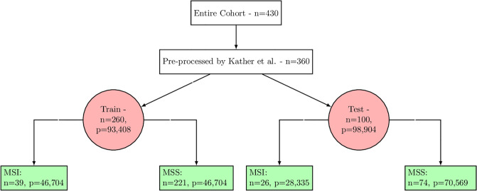
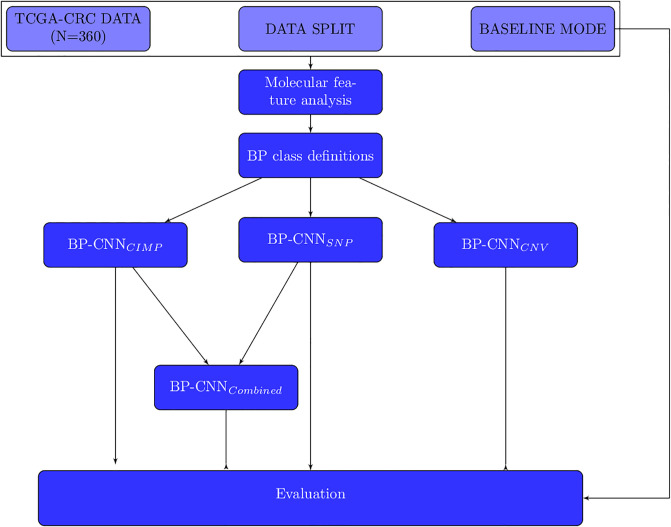
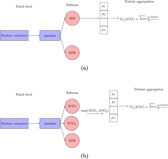
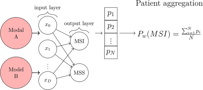
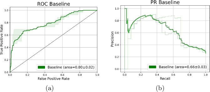
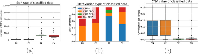
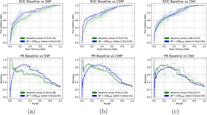
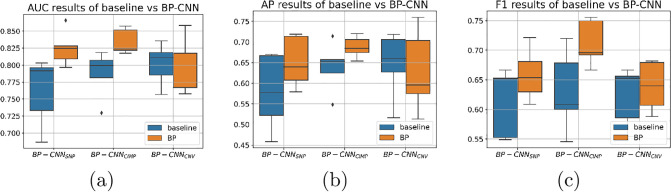
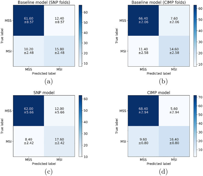
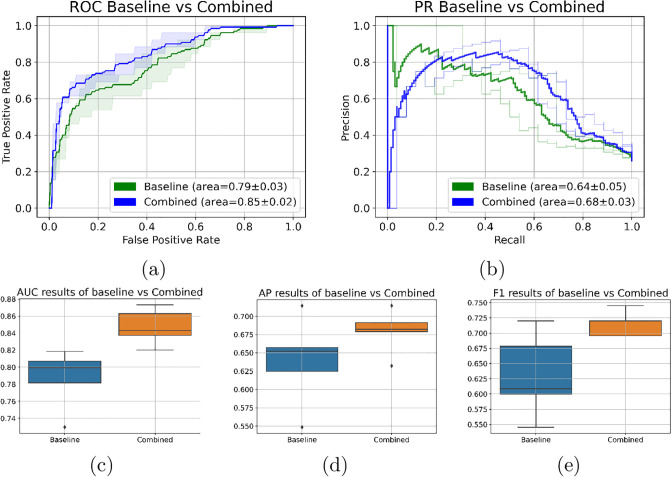
Molecular subtypes of colorectal cancer (CRC) significantly influence treatment decisions. While convolutional neural networks (CNNs) have recently been introduced for automated CRC subtype identification using H&E stained histopathological images, the correlation between CRC subtype genomic variants and their corresponding cellular morphology expressed by their imaging phenotypes is yet to be fully explored. The goal of this study was to determine such correlations by incorporating genomic variants in CNN models for CRC subtype classification from H&E images. We utilized the publicly available TCGA-CRC-DX dataset, which comprises whole slide images from 360 CRC-diagnosed patients (260 for training and 100 for testing). This dataset also provides information on CRC subtype classifications and genomic variations. We trained CNN models for CRC subtype classification that account for potential correlation between genomic variations within CRC subtypes and their corresponding cellular morphology patterns. We assessed the interplay between CRC subtypes' genomic variations and cellular morphology patterns by evaluating the CRC subtype classification accuracy of the different models in a stratified 5-fold cross-validation experimental setup using the area under the ROC curve (AUROC) and average precision (AP) as the performance metrics. The CNN models that account for potential correlation between genomic variations within CRC subtypes and their cellular morphology pattern achieved superior accuracy compared to the baseline CNN classification model that does not account for genomic variations when using either single-nucleotide-polymorphism (SNP) molecular features (AUROC: 0.824±0.02 vs. 0.761±0.04, p<0.05, AP: 0.652±0.06 vs. 0.58±0.08) or CpG-Island methylation phenotype (CIMP) molecular features (AUROC: 0.834±0.01 vs. 0.787±0.03, p<0.05, AP: 0.687±0.02 vs. 0.64±0.05). Combining the CNN models account for variations in CIMP and SNP further improved classification accuracy (AUROC: 0.847±0.01 vs. 0.787±0.03, p = 0.01, AP: 0.68±0.02 vs. 0.64±0.05). The improved accuracy of CNN models for CRC subtype classification that account for potential correlation between genomic variations within CRC subtypes and their corresponding cellular morphology as expressed by H&E imaging phenotypes may elucidate the biological cues impacting cancer histopathological imaging phenotypes. Moreover, considering CRC subtypes genomic variations has the potential to improve the accuracy of deep-learning models in discerning cancer subtype from histopathological imaging data.
Copyright: © 2024 Hezi et al. This is an open access article distributed under the terms of the Creative Commons Attribution License, which permits unrestricted use, distribution, and reproduction in any medium, provided the original author and source are credited.
Conflict of interest statement
The authors have declared that no competing interests exist.
Figures
Similar articles
-
CIMIL-CRC: A clinically-informed multiple instance learning framework for patient-level colorectal cancer molecular subtypes classification from H&E stained images.Comput Methods Programs Biomed. 2025 Feb;259:108513. doi: 10.1016/j.cmpb.2024.108513. Epub 2024 Nov 19. Comput Methods Programs Biomed. 2025. PMID: 39581068
-
Development and validation of a weakly supervised deep learning framework to predict the status of molecular pathways and key mutations in colorectal cancer from routine histology images: a retrospective study.Lancet Digit Health. 2021 Dec;3(12):e763-e772. doi: 10.1016/S2589-7500(21)00180-1. Epub 2021 Oct 19. Lancet Digit Health. 2021. PMID: 34686474 Free PMC article.
-
Color-CADx: a deep learning approach for colorectal cancer classification through triple convolutional neural networks and discrete cosine transform.Sci Rep. 2024 Mar 22;14(1):6914. doi: 10.1038/s41598-024-56820-w. Sci Rep. 2024. PMID: 38519513 Free PMC article.
-
Deep learning for colon cancer histopathological images analysis.Comput Biol Med. 2021 Sep;136:104730. doi: 10.1016/j.compbiomed.2021.104730. Epub 2021 Aug 4. Comput Biol Med. 2021. PMID: 34375901 Review.
-
Classification of colorectal cancer based on correlation of clinical, morphological and molecular features.Histopathology. 2007 Jan;50(1):113-30. doi: 10.1111/j.1365-2559.2006.02549.x. Histopathology. 2007. PMID: 17204026 Review.
Cited by
-
Accurate colorectal cancer detection using a random hinge exponential distribution coupled attention network on pathological images.Abdom Radiol (NY). 2025 Jul;50(7):2828-2857. doi: 10.1007/s00261-024-04770-2. Epub 2025 Jan 8. Abdom Radiol (NY). 2025. PMID: 39779530
References
-
- Sung H, Ferlay J, Siegel RL, Laversanne M, Soerjomataram I, Jemal A, et al.. Global cancer statistics 2020: GLOBOCAN estimates of incidence and mortality worldwide for 36 cancers in 185 countries. CA: a cancer journal for clinicians. 2021;71(3):209–249. - PubMed
-
- He K, Zhang X, Ren S, Sun J. Deep residual learning for image recognition. In: Proceedings of the IEEE conference on computer vision and pattern recognition; 2016. p. 770–778.
MeSH terms
LinkOut - more resources
Full Text Sources
Medical
