ARViS: a bleed-free multi-site automated injection robot for accurate, fast, and dense delivery of virus to mouse and marmoset cerebral cortex

Abstract

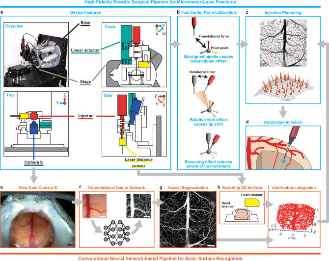
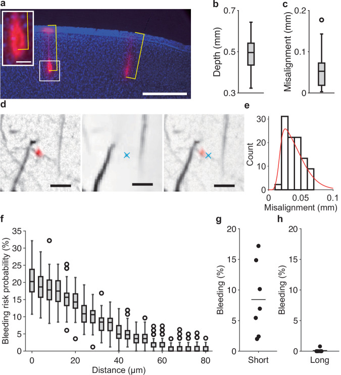
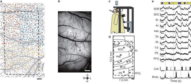
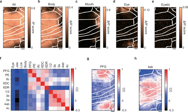
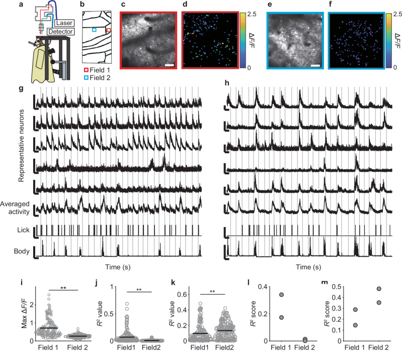
Genetically encoded fluorescent sensors continue to be developed and improved. If they could be expressed across multiple cortical areas in non-human primates, it would be possible to measure a variety of spatiotemporal dynamics of primate-specific cortical activity. Here, we develop an Automated Robotic Virus injection System (ARViS) for broad expression of a biosensor. ARViS consists of two technologies: image recognition of vasculature structures on the cortical surface to determine multiple injection sites without hitting them, and robotic control of micropipette insertion perpendicular to the cortical surface with 50 μm precision. In mouse cortex, ARViS sequentially injected virus solution into 100 sites over a duration of 100 min with a bleeding probability of only 0.1% per site. Furthermore, ARViS successfully achieved 266-site injections over the frontoparietal cortex of a female common marmoset. We demonstrate one-photon and two-photon calcium imaging in the marmoset frontoparietal cortex, illustrating the effective expression of biosensors delivered by ARViS.

Fig. 1. Workflow of an automated injection.

a Device picture and schematic of the device features. An injector (red), a linear actuator (green), a laser distance sensor (yellow), and Camera S (blue) were mounted on the stage of a six-axis hexapod. The animal’s head was fixed in the apparatus on the base plate (the animal is not shown). Light orange, blue, and red arrows shown in the upper right of each inset represent the X, Y, and Z axes in the robot base system frame, respectively. The V (orange) and W (green) rotation directions are also shown. b Schematic of tool center point calibration. Top, any misalignment of the pipette tip position from the pivot point can cause an unintended translational offset from the desired position. Middle, when the pipette rotates around the pivot point, this offset can induce an unexpected shift in the position of the pipette tip. Bottom, minimizing this offset is essential for 3D manipulation of the micropipette. c, A representation of multiple injection sites (red points) on the mouse cortical surface with vessel segmentation (black) and the pipette insertion directions (red lines in the bottom). The injection site positions and pipette angles are designed based on data from the surface recognition pipeline (e–i). d Illustration of the automated injection into the target point within the cortical tissue. e A representative image of the mouse cortical surface captured by Camera S shown in (a). Scale bar, 1 mm. f Schematic of the segmentation of blood vessels on the cortical surface with a convolutional neural network. An example pair of input and output images are shown on the left and right, respectively. Scale bars, 1 mm. g A representative stitched image of the vessel segmentation over the whole dorsal cortex of a mouse. Scale bar, 1 mm. h Schematic of 3D cortical surface scanning with the laser distance sensor. i An example of the projection of the vessel pattern onto the 3D cortical surface. Source data are provided as the Source Data file.

Fig. 2. Vessel segmentation on the cortical surface.

a An example input image of the mouse cortical surface for SA-UNet. Scale bar, 1 mm. b Example output images of vessel segmentation in the DRIVE model (left), the initial model (middle), and the final model (right). The input image is the image shown in (a). Scale bar, 1 mm. Some parts of thick vessels were only segmented in the final model (arrows). c Left, an example image of the cortical surface captured by the microscope with a 5× magnification objective. Middle, manually created vessel segmentation of the left image. Right, skeletonized blood vessel mask of the middle image. The color of the skeleton corresponds to the width of the vessel at the corresponding point. Scale bar, 0.3 mm. d Left, an image captured by Camera S. The imaged area is the same as in (c). Middle, a vessel mask of the left image generated by the final model. Right, skeletonized blood vessel mask of the middle image. Vessels overlaid by the mask in (c) are shown in red, while the rest are in blue. Scale bar, 0.3 mm. e Histogram of the total lengths of the vessels that were detected on the 5× magnification image (blue) and those that were recognized by the final model (red) for each bin width. A black plot for each bin width indicates the ratio of the latter length to the former length (n = 1 mouse). Source data are provided as the Source Data file.

Fig. 3. Determination of multiple injection sites in the two-dimensional vessel segmentation image.

a Schematic of the transformation process from the original stitched image to the YZ stitched image. Left: Each image was acquired by adjusting the X position so that the position of the reference point where the pipette tip should be imaged matched the cortical surface, and these images were then stitched to form the original stitched image (Y_camera-Z_camera plane). Circles on the cortical surface indicate the reference points and circles on the stitched images are their projection. Middle: By inferring the angle between the camera and laser optical axes, the original stitched image was mapped to the corresponding cortical surface with geometric transformation. Right: The image mapped on the cortical surface was projected to the YZ plane as the YZ stitched image. The camera angle and the curvature of the cortical surface are more emphatic than factual. b Representative overlay of the vessel segmentations of the original stitched image (magenta) and the YZ stitched image (green). Scale bar, 1 mm. c Diagram for the injection site planning algorithm. The initial number (n = 71 in this mouse) of sites (black dots) within the safety regions (colors) were determined according to the k-means clustering method. Different colors indicate different clusters. White areas indicate the safety margin region (with a safety margin distance of 65 μm in this mouse) and blood vessels. Next, two sites whose cluster areas including blood vessels were the smallest and second smallest (red dots) were removed and one new site was added. After these procedures were repeated approximately 10 times (eleven times in this mouse), the target injection sites were determined. Scale bar, 1 mm. d Histogram of the distance between the target injection site and the corresponding nearest neighbor site (n = 679 sites from seven mice). e Histogram of the distance between the target injection site and the corresponding nearest blood vessel (n = 679 sites from seven mice). Source data are provided as the Source Data file.

Fig. 4. Tool center point (TCP) calibration.

a Schematic of a binocular camera system for the 3D reconstruction of the pipette tip coordinates. 3D coordinates of the pipette tip are inferred from two 2D coordinates from the Camera L image (X^L, Y^L) and Camera R image (X^R, Y^R). b Example images of the glass micropipette captured by Camera L (left) and Camera R (right). The images were filtered, and the contrast was adjusted. Scale bar, 1 mm. c, Coordinate system used for solving the tool center point calibration problem. ${\mathrm{P}}_{\mathrm{Pipette}}^{\mathrm{E}}$ is a vector that indicates the initial position of the pipette tip in frame {E}. Light orange, X axis; cyan, Y axis; red, Z axis. The directions of V (orange) and W (green) rotations are also shown. d, e Representative plots of estimated pipette tip coordinates relative to the original tip coordinates before (d) and after (e) MSAC algorithm implementation. Only the coordinates regarded as inliers with the MSAC algorithm are shown for comparison (n = 131). The pseudo-color bar indicates the distance between the estimated pipette movement and the scheduled movement of the robot. f Histogram of the distance between the estimated pipette movement and scheduled movement of the robot without (orange) and with (blue) the MSAC algorithm. g A representative map of the pipette tip shift resulting from specific V and W rotation patterns before compensation for rotation error. h A representative map of the pipette tip shift resulting from specific V and W rotation patterns after the first part of the compensation for rotation error. i X- (left), Y- (middle), and Z- (right) axial maps of the pipette tip shift of the map shown in (h) after the interpolation using the thin-plate spline method. j A map of the pipette tip shift resulting from specific V and W rotation patterns after the compensation for rotation error. k Histogram of the pipette tip shift for rotations with only conventional TCP calibration (orange), with grid searching after TCP calibration (green), and with all methods including the compensation (blue). Source data are provided as the Source Data file.

Fig. 5. The accuracy of the pipette injection in vivo.

a, A representative coronal section of the post-fixed cerebral cortex of a mouse into which fluorescent dye (CM-DiI; red) was injected. The section was Nissl-stained (blue). The yellow lines indicate the depth of the injection from the cortical surface. When the putative pipette location was considered as a black void surrounded by the fluorescent dye, the deepest point of the void was measured as the depth of the injection (inset). Otherwise, the injection’s depth was determined by measuring the deepest point of the fluorescent dye. Scale bar, 0.5 mm. Scale bar in the inset, 50 µm. b Box-and-whisker diagram of the measured depth (n = 32 sites from one mouse). c Box-and-whisker diagram of the absolute difference between the targeted and measured depths (n = 32 sites from one mouse). For panel (b, c), the center line, box limits and whiskers denote the median, quartiles, and 1.5 × interquartile ranges in the boxplot, respectively. d Representative images showing the lateral misalignment of the pipette injection site. Left: A fluorescence (red, CM-DiI) image of the actual injection site superimposed on a bright field image. Middle: The target injection site (a blue cross) superimposed on a bright field image of the SA-UNet segmentation. Right: A composite image of the left and middle images. Scale bar, 100 μm. e Histogram of the lateral misalignment of the pipette tip (n = 32 sites from one mouse). The red curve indicates a non-parametric approximation of the lateral misalignment distribution, calculated using a Gaussian kernel. f Box-and-whisker diagram of the bleeding risk probability against the safety margin distance (n = 100 simulations). The center line, box limits and whiskers denote the median, quartiles, and 1.5 × interquartile ranges in the boxplot, respectively. g, h Rates of short (g) and long (h) bleeding when the pipette was injected perpendicular to the cortical surface at each site (n = 7 mice). The horizontal line represents the mean. Source data are provided as the Source Data file.

Fig. 6. Wide-field calcium imaging of the frontoparietal cortex in an awake marmoset.

a A vascular image of the marmoset frontoparietal cortex that was segmented by the SA-UNet (in gray) with target injection sites (colored dots). Blue, red, and yellow dots represent the first, second, and third sections, respectively. The black dashed frame represents the field of view for the fluorescence microscopy. The slightly distorted shape was caused by the affine transformation of the frame shown in (b), which was based on the blood vessel structure. This might be due to the elapsed time from the injection and distortion of the cortex caused by installation of the glass window. Scale bar, 1 mm. b Fluorescence image of the same area as (a) 7 weeks after the virus injection. Scale bar, 1 mm. A, P, M, and L stand for anterior, posterior, medial, and lateral, respectively. c Schematic of the experimental setup for wide-field one-photon calcium imaging of the marmoset in an awake head-fixed condition. d Putative cortical areas within the imaging window (black frame). The dashed frame indicates the field of view (14.2 × 7.2 mm). Parcellation is based on the stereotaxic atlas and ICMS (see Supplementary Fig. 8c). Small black squares represent ROIs for the corresponding cortical areas. Scale bar, 1 mm. e Representative time courses of ∆F/F at the ROIs of ten cortical areas shown in (c), licking, and body movement. The vertical gray lines show the reward timing. The vertical scale bars on the fluorescence traces represent 0.1 ∆F/F. The vertical scale bars with a lick represent a binary value of 1 and those with normalized body movement represent an intensity value of 1. The horizontal scale bars represent 5 s. The blue bars at the top indicate the quiet periods, whereas the yellow bars at the top indicate the periods outside of the quiet periods. Source data are provided as the Source Data file.

Fig. 7. Movement representations and activity correlations in the marmoset frontoparietal cortex.

a Spatial map of the accuracy (R²) of the encoding model for predicting the neural activity with all behavioral variables. The pseudo-colors represent R² values. Scale bar for (a–e), 1 mm. b–e Spatial maps of the unique contribution (ΔR²) of the body (b), mouth (c), eye (d), and eyelid (e) variables to the explanation of the neural activity. The pseudo-colored bar represents the ΔR² score. f Correlation matrix during the quiet periods between the cortical areas and movement variables (left), and between cortical areas (right). Two clusters between cortical areas were determined using hierarchical clustering. The pseudo-colored bar represents the correlation coefficient (CC). Note that although the eye movement was not considered in the definition of the quiet periods, all neuronal activity showed very weak correlations with eye movement. g, h Correlation maps between seed pixels (indicated by white filled circles) located in area PFG (g) and area 4ab (h) with the other pixels. The pseudo-colored bar represents the correlation coefficient (CC). Source data are provided as the Source Data file.

Fig. 8. Two-photon calcium imaging of movement-related neurons in the marmoset motor cortex.

a Schematic of the experimental setup to perform two-photon calcium imaging in the awake condition. b, Locations of two fields (red for field 1 and blue for field 2) in which two-photon imaging was conducted. c, e Time-averaged and contrast-adjusted two-photon images for field 1 (c) and field 2 (e). Scale bars, 100 µm. d, f Neuronal somata extracted by the CNMF algorithm (Pnevmatikakis et al., 2016) from field 1 (d) and field 2 (f). Each neuronal soma is colored according to the maximum value from the trial-averaged ΔF/F trace during the period spanning 1 s before to 8 s after the reward timing. g, h Representative traces of five neurons from field 1 (g) and field 2 (h), averaged activity of all active neurons in each field, lick frequency, and body movement. The vertical gray lines show the reward timing. The vertical scale bars with the fluorescence traces, averaged activity, lick, and movement represent 500% ∆F/F, 100% ΔF/F, an intensity value of 1 (arb. unit), and an intensity value of 5 (pixel), respectively. The horizontal scale bars represent 10 s. i Maximum values of trial-averaged ΔF/F traces for a period spanning 1 s before to 8 s after the reward timing in field 1 (red, n = 159 from two sessions) and field 2 (blue, n = 182 from two sessions). Horizontal bars indicate the means. **p = 5.0 × 10^–23, two-sided Welch’s test. j, k The prediction accuracy (R²) of individual neurons in fields 1 (red, n = 159 from two sessions) and 2 (blue, n = 182 from two sessions) for the licking frequency (j) and body movement (k). Horizontal bars indicate the means. **p = 2.6 × 10^–10 (j) and 0.0028 (k), one-sided Welch’s test. l, m The prediction accuracy (R²) of the averaged activity in fields 1 (n = two sessions) and 2 (n = two sessions) for the lick frequency (l) and body movement (m). Source data are provided as the Source Data file.

References

1. Tian, L. et al. Imaging neural activity in worms, flies and mice with improved GCaMP calcium indicators. Nat. Methods6, 875–881 (2009). 10.1038/nmeth.1398 - DOI - PMC - PubMed
1. Grienberger, C. & Konnerth, A. Imaging Calcium in Neurons. Neuron73, 862–885 (2012). 10.1016/j.neuron.2012.02.011 - DOI - PubMed
1. Miyawaki, A. et al. Fluorescent indicators for Ca2+based on green fluorescent proteins and calmodulin. Nature388, 882–887 (1997). 10.1038/42264 - DOI - PubMed
1. Marvin, J. S. et al. Stability, affinity, and chromatic variants of the glutamate sensor iGluSnFR. Nat. Methods15, 936–939 (2018). 10.1038/s41592-018-0171-3 - DOI - PMC - PubMed
1. Sun, F. et al. A genetically encoded fluorescent sensor enables rapid and specific detection of dopamine in flies, fish, and mice. Cell174, 481–496.e19 (2018). 10.1016/j.cell.2018.06.042 - DOI - PMC - PubMed
Publication types
LinkOut - more resources