A whole-body micro-CT scan library that captures the skeletal diversity of Lake Malawi cichlid fishes

Abstract

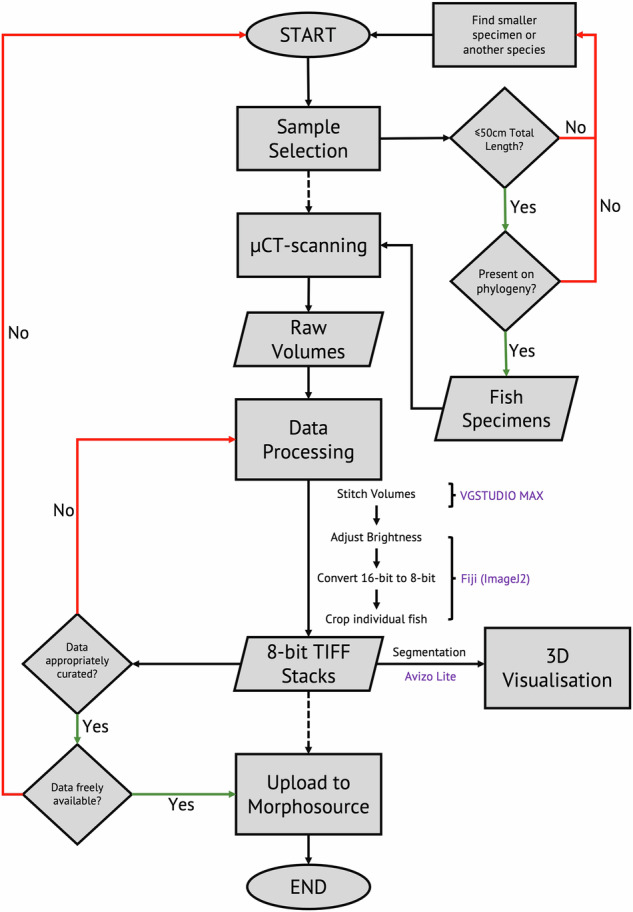
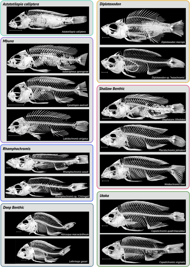
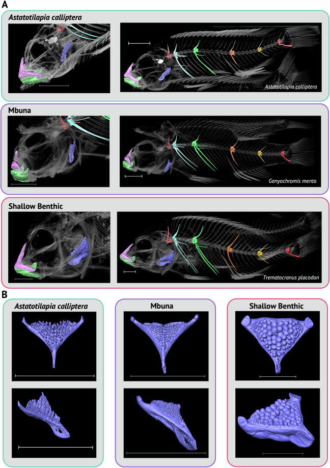
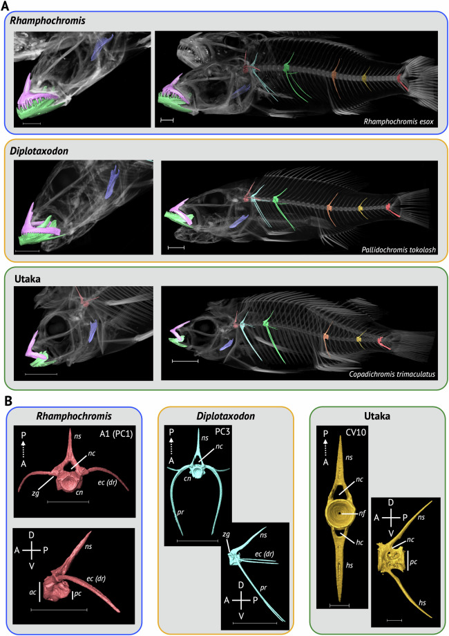
Here we describe a dataset of freely available, readily processed, whole-body μCT-scans of 56 species (116 specimens) of Lake Malawi cichlid fishes that captures a considerable majority of the morphological variation present in this remarkable adaptive radiation. We contextualise the scanned specimens within a discussion of their respective ecomorphological groupings and suggest possible macroevolutionary studies that could be conducted with these data. In addition, we describe a methodology to efficiently μCT-scan (on average) 23 specimens per hour, limiting scanning time and alleviating the financial cost whilst maintaining high resolution. We demonstrate the utility of this method by reconstructing 3D models of multiple bones from multiple specimens within the dataset. We hope this dataset will enable further morphological study of this fascinating system and permit wider-scale comparisons with other cichlid adaptive radiations.

Fig. 1

A summary of the μCT-scan dataset. We were able to sample species from all seven ecomorphological groups in the Lake Malawi haplochromine radiation. The phylogenetic relationships between the majority of the species scanned is indicated and coloured according to the respective ecomorphology. The tree is a pruned version of the full (no intermediates) neighbour-joining tree published by Malinsky et al., which is rooted to Neolamprologous brichardi, a non-haplochromine cichlid endemic to Lake Tanganyika. Longer terminal branches reflect a higher ratio of within-species to between-species variation. A cladogram depicting the relationship between the Lake Victoria, Lake Malawi and the Astatotilapia species native to the Great Ruaha River is indicated in the black box. We also scanned 18 species of cichlid whose phylogenetic relationships are not resolved in the phylogeny shown. The names of these species, most of which are undescribed, are indicated in their respective ecomorphological group in bold. Pictures (not to scale) of example species belonging to each ecomorphological group are also shown. Black bar: 2 × 10⁻⁴ substitutions per base pair. Fish images used with permission from Ad Konings (Alticorpus macrocleithrum, Diplotaxodon greenwoodi, Genyochromis mento, Hemitilapia oxyrhynchus, Iodotrophesus sprengerae, Nimbochromis polystigma, Placidochromis milomo and Trematocranus placodon), George F. Turner (Astatotilapia sp. ‘Ruaha blue’, Diplotaxodon macrops, Mylochromis anaphyrmus, Otopharynx speciosus and Rhamphochromis woodi), Martin J. Genner (Diplotaxodon sp. ‘similis white-back north’, Diplotaxodon sp. ‘macrops ngulube’ and Rhamphochromis sp. ‘Chilingali’), Hannes Svardal (Copadichromis virginalis) and Callum V. Bucklow (Maylandia zebra). Fish images are not to scale.

Fig. 2

Flowchart of μCT-scanning, image processing and segmentation methodology. The flowchart outlines the necessary decisions that were made during collation of the described μCT scan dataset. Rectangles represent processes; parallelograms represent inputs or outputs; diamonds represent decisions. It is sufficiently generalised that it can be reused for future data collection. We were focused on generating data for a specific macroevolutionary study, so we restricted the dataset to species with known phylogenetic placements but this is not strictly necessary. Software associated with data processing steps are indicated in purple. Further information about processing and segmentation is provided in the Usage Notes.

Fig. 3

Specimen preparation for μCT-scanning. Multiple fish were scanned at the same time (A). Individual fish were labelled and placed in separate plastic bags so they could be correctly identified and stored after imaging (B). Unique objects (C) that would be readily identifiable following μCT-scanning were attached to the outside of these bags, ideally close to the heads, positioned outwards (F, arrows), and bundled together with tape (D–F) all with the same orientation (head-up). Bundles were then wrapped in bubble wrap and other packaging material (G,H) and tightly sealed inside a plastic container, again head-up (I). Containers were left for at least ten minutes to settle to prevent movement during scanning (J) and an additional label was placed on the container to permit future identification if multiple batches were prepared together (K).

Fig. 4

Whole-body 3D models of select specimens from the dataset. Specimens are arranged according to the ecomorphological group they belong to. Species names are indicated. The ring structure in Diplotaxodon sp. ‘holochromis’ and Lethrinops gossei is a rubber band used for identification purposes. Scale for all images is shown as 1cm. See Supplementary Table S1 for details of the specimens used.

Fig. 5

Segmented Bones from Astatotilapia calliptera, Genyochromis mento (mbuna) and Trematocranus placodon (shallow benthic). (A, left) A close up, lateral view of the head of each species (species name indicated on right), showing the dentary (green), premaxilla (pink) and lower pharyngeal jaw (purple) positioned within a volume render of the head. (A, right) A whole body lateral view showing the aforementioned jaw bones, as well as the first non-rib-bearing vertebra (orange), the first rib-bearing (precaudal, PC) vertebrae (light blue), PC8 (green), non-rib bearing (caudal, CV), CV3 (orange), CV10 (gold) and the pre-urostyle vertebrae (red). (B) Anterior (top) and anterolateral (bottom) view of the lower pharyngeal jaws for each species in (A). Scale for all images is 1cm. See Supplementary Table S1 for details of the specimens used. 3D models for all segmented bones can be found in the Supplementary Material.

Fig. 6

Segmented Bones from Rhamphochromis esox (Rhamphochromis), Pallidochromis tokolosh (Diplotaxodon) and Copadichromis trimaculatus (Utaka). (A) Left, lateral view of the head of each species, showing the dentary (green), premaxilla (pink) and lower pharyngeal jaw (purple). Right, whole body lateral views showing aforementioned jaw bones, as well as the first non-rib-bearing vertebrae (orange), the first rib-bearing (precaudal, PC) vertebrae (light blue), PC8 (green), non-rib bearing (caudal, CV), CV3 (orange), CV10 (gold) and the pre-urostyle vertebrae (red). (B) Images of select vertebrae (indicated) from each species shown in (A). Axes are indicated (A, anterior; P, posterior; D, dorsal; V, ventral). Vertebral models are labelled (ac, anterior cone span; cn, centrum; ec (dr), epicentrals (dorsal ribs); hc, haemal canal; hs, haemal spine; nc, neural canal; nf, neural foramen; ns, neural spine; pc, posterior cone span; pr, pleural ribs; zg, zygapophyses). Scale for all images is 1cm, besides CV10 for Utaka which is 0.1cm. See Supplementary Table S1 for details of the specimens used. 3D models for all segmented bones can be found in the supplementary material.

Fig. 7

Example specimen volume rendering with body aspect ratio landmarks. The number of precaudal (pink) and caudal vertebrae (blue), including the urostyle, the total number of vertebrae (sum of the precaudal and caudal vertebrae, including the urostyle) and the body aspect ratio was estimated for 113 of the 116 specimens in the dataset. The landmarks used to estimate the body aspect ratio are indicated in the figure on an example specimen (Maylandia zebra, L-BV:M6, see Supplementary Table S1). Landmarks 1 and 2 were used to calculate the length, and landmarks 3 and 4 the width by calculating the length of a straight line between the x,y coordinates. Landmark 1, anterior tip of the premaxilla; Landmark 2, centre of the urostyle; Landmark 3, Base of the first dorsal fin spine; Landmark 4, base of the pelvic fin spine.

References

1. Turner, G. F., Seehausen, O., Knight, M. E., Allender, C. J. & Robinson, R. L. How many species of cichlid fishes are there in African lakes? Molecular Ecology10, 793–806, 10.1046/j.1365-294x.2001.01200.x (2001). 10.1046/j.1365-294x.2001.01200.x - DOI - PubMed
1. Barlow, G. The Cichlid Fishes: Nature’s Grand Experiment In Evolution (Hachette UK, London, 2008).
1. Sparks, J. S. & Smith, W. L. Phylogeny and biogeography of cichlid fishes (Teleostei: Perciformes: Cichlidae). Cladistics20, 501–517, 10.1111/j.1096-0031.2004.00038.x (2004). 10.1111/j.1096-0031.2004.00038.x - DOI - PubMed
1. Malinsky, M. et al. Whole-genome sequences of Malawi cichlids reveal multiple radiations interconnected by gene flow. Nature Ecology I& Evolution2, 1940–1955, 10.1038/s41559-018-0717-x (2018). 10.1038/s41559-018-0717-x - DOI - PMC - PubMed
1. Svardal, H. et al. Ancestral hybridization facilitated species diversification in the Lake Malawi cichlid fish adaptive radiation. Molecular biology and evolution37, 1100–1113, 10.1093/molbev/msz294 (2020). 10.1093/molbev/msz294 - DOI - PMC - PubMed
Publication types
LinkOut - more resources