Disease prediction with multi-omics and biomarkers empowers case-control genetic discoveries in the UK Biobank

Abstract

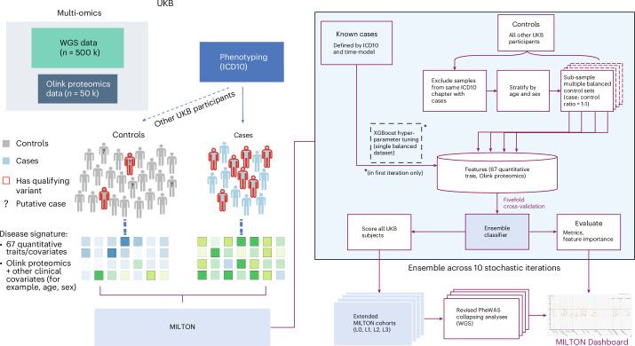
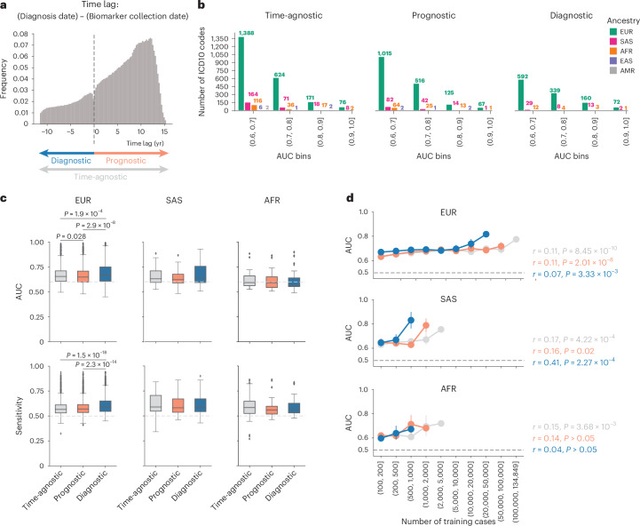
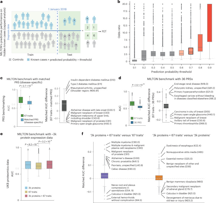
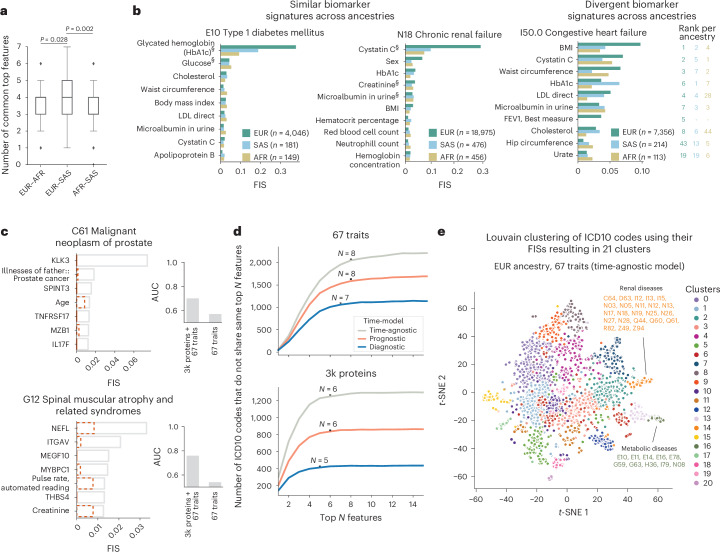
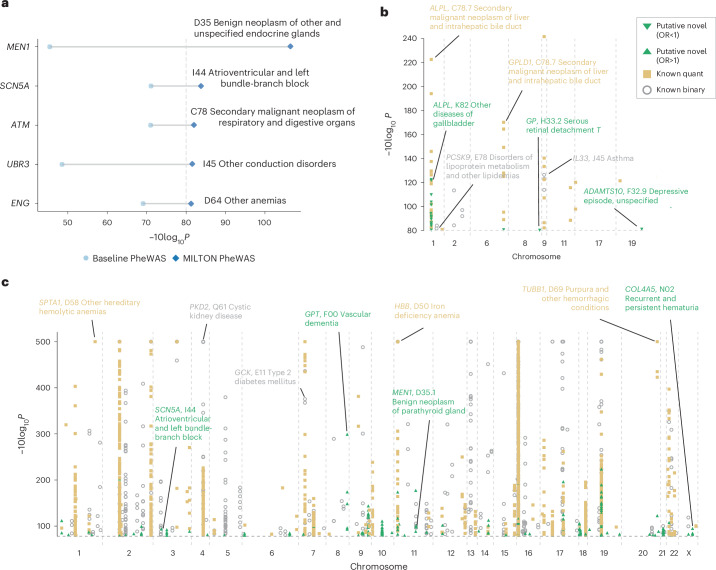
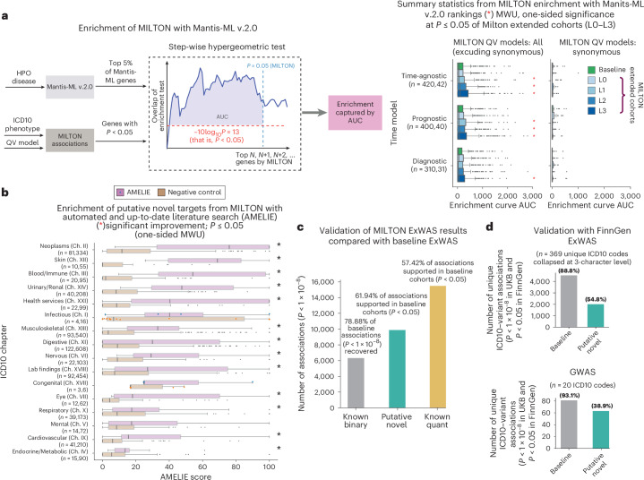
The emergence of biobank-level datasets offers new opportunities to discover novel biomarkers and develop predictive algorithms for human disease. Here, we present an ensemble machine-learning framework (machine learning with phenotype associations, MILTON) utilizing a range of biomarkers to predict 3,213 diseases in the UK Biobank. Leveraging the UK Biobank's longitudinal health record data, MILTON predicts incident disease cases undiagnosed at time of recruitment, largely outperforming available polygenic risk scores. We further demonstrate the utility of MILTON in augmenting genetic association analyses in a phenome-wide association study of 484,230 genome-sequenced samples, along with 46,327 samples with matched plasma proteomics data. This resulted in improved signals for 88 known (P < 1 × 10^-8) gene-disease relationships alongside 182 gene-disease relationships that did not achieve genome-wide significance in the nonaugmented baseline cohorts. We validated these discoveries in the FinnGen biobank alongside two orthogonal machine-learning methods built for gene-disease prioritization. All extracted gene-disease associations and incident disease predictive biomarkers are publicly available ( http://milton.public.cgr.astrazeneca.com ).

Fig. 1. MILTON flowchart.

Individuals diagnosed with certain ICD10 codes in the UKB are herein referred to as ‘cases’ and all remaining individuals as ‘controls’ for that ICD10. Both cases and controls can have QVs, such as protein truncating variants, in a given gene. The objective of rare-variant collapsing analysis is to identify genes in which QVs are enriched in either cases or controls. Some controls may not yet be diagnosed with a given ICD10 code or are incorrectly classified. MILTON aims to identify these individuals by checking if they share similar biomarker profiles to known cases (represented by the shades of green). The predicted cases are eventually merged with the known cases to form an ‘augmented case cohort’ (ranging from ‘L0’ to ‘L3’), which is analyzed along with a revised control set in an updated PheWAS on whole-genome sequencing (WGS) data.

Fig. 2. MILTON time-models and phenome-wide performance across ancestries.

a, Schematic showing how different time-models are defined and the frequency of individuals that had biomarker sample collection certain years before or after diagnosis date. Diagnosis dates recorded in UKB fields 41280, 40000 or 40005 were taken for each individual (Methods). b, MILTON AUC performance across all ICD10 codes, five ancestries and three time-models. c, Comparison of median AUC and sensitivity performance of MILTON models across ten replicates trained on 1,466, 73 and 56 ICD10 codes under EUR, SAS and AFR ancestries, respectively, and different time-models. MWU, two-sided P values are shown. Each box plot shows the median as center line, 25th percentile as lower box limit and 75th percentile as upper box limit, and whiskers extend to 25th percentile − 1.5 × interquartile range at the bottom and 75th percentile + 1.5 × interquartile range at the top; points denote outliers. d, Distribution of median AUC across ten replicates with increasing number of training cases per ICD10 code across different time-models and ancestries. Error-bar represents 95% confidence interval with center representing mean statistic. Pearson correlation coefficients (r) and two-sided P values (P) for each time-model are provided. Source data

Fig. 3. MILTON validation and benchmarks with proteomics data and PRSs.

a, Overview of capped analysis. Here, all individuals diagnosed until 1 January 2018 were used during model training and all individuals diagnosed thereafter were used as the test set for predictions. A 2 × 2 contingency table was constructed to capture whether known cases and controls were eventually correctly predicted by MILTON. b, Distribution of odds ratio obtained from Fisher’s exact test (FET) in capped analysis on 1,748 ICD10 codes across multiple prediction probability thresholds, indicating the power of MILTON to predict known cases hidden from the training set. Results with predicted probability threshold ≥ 0.6 are filled with orange color and those corresponding to threshold = 0.7 are highlighted in black boundary. c, Performance comparison of MILTON time-agnostic models when trained on 67 traits versus disease-specific PRSs across 151 ICD10 codes. d, Box plots comparing the performance of MILTON time-agnostic models when trained on 67 traits versus all 36 PRSs across 499 ICD10 codes. e, Performance comparison of MILTON time-agnostic models when trained on protein expression data + covariates ± 67 traits versus 67 traits across 1,574 ICD10 codes (Methods). f, AUC differences when MILTON is trained on different feature set combinations for 1,299 ICD10 codes (time-agnostic model). Left, x axis represents median AUC_{3k proteins+67 traits} − median AUC_{67 traits} for matched ICD10 codes. Right, x axis represents median AUC_{3k proteins+67 traits} − median AUC_{3k proteins} for matched ICD10 codes. In b–f, each box plot shows median as center line, 25th percentile as lower box limit and 75th percentile as upper box limit; whiskers extend to 25th percentile − 1.5× interquartile range at the bottom and 75th percentile + 1.5× interquartile range at the top; points denote outliers. MWU, two-sided P values are shown in c–e. Source data

Fig. 4. Overview of most important biomarker features learnt by MILTON per ICD10 code for time-agnostic models.

a, Number of top seven biomarkers shared between each pair of ancestries for all 149 ICD10 codes with AUC > 0.6. MWU, two-sided P values are shown. No multiple testing correction was performed. Box plot shows median as center line, 25th percentile as lower box limit and 75th percentile as upper box limit; whiskers extend to 25th percentile − 1.5× interquartile range at the bottom and 75th percentile + 1.5 × interquartile range at the top; points denote outliers. b, Features with the highest FISs for E10 (type 1 diabetes mellitus), N18 (chronic renal failure) and I50.0 (congestive heart failure) for each ancestry. ^§Biomarkers that were also listed by an expert for given disease area. LDL, low-density lipoprotein; FEV1, forced expiratory volume in 1 s. c, Top predictive features for C61 and G12 when using UKB proteomics data to train MILTON (time-agnostic model). Dashed, orange bar plots indicate average FIS of corresponding feature across all ICD10 codes for time-agnostic model. Bar plots comparing AUC between models trained on proteomics data along with 67 traits versus 67 traits only are shown on the right. d, Number of ICD10 codes that do not share the top N features as a function of N, indicating a quasi-unique biomarker signature per disease, comprising N ≥ 7 features when models are trained on 67 features only and N ≥ 5 features when models are trained on proteomics data only. e, The t-distributed stochastic neighbor embedding (t-SNE) projection of diseases across the phenome based on their MILTON-derived FISs. Each point corresponds to an ICD10 code, colored by Louvain clustering. Source data

Fig. 5. PheWAS results on MILTON-augmented cohorts, based on whole-genome sequencing data, and stratification across known and putative novel hits.

a, Examples of known gene–disease associations from literature that reached genome-wide significance via MILTON. b,c Manhattan plots showing the distribution of gene–ICD10 associations with odds ratio (OR) < 1 (b) and OR > 1 (c) across different chromosome positions. For a–c, FET was used to calculate P values and odds ratios (two-sided, unadjusted). Source data

Fig. 6. Validation of PheWAS results on MILTON-augmented cohorts using orthogonal machine-learning methods and FinnGen.

a, Left, flowchart depicting the stepwise hypergeometric tests performed to test enrichment of top predictions between MILTON-based PheWAS results (FET, two-sided, unadjusted P < 0.05) and top gene–disease associations predicted by Mantis-ML (v.2.0; Methods). Right, box plots comparing the enrichment AUC between MILTON-augmented cohorts and baseline cohorts across all three time-models and across all nonsynonymous QV models or exclusively on the synonymous QV model. Number of samples shown refers to these cases. Comparison is done for 14 HPO terms that could be manually mapped to ICD10 codes. b, Breakdown of AMELIE-aggregated scores by ICD10 chapter (sorted by chapter median) for putative novel targets per three-character ICD10 code. Negative controls were generated through ten samplings of random gene sets, equal in size to the respective MILTON gene sets. Points are plotted only for boxes where n < 10. c, Validation of MILTON ExWAS results, and putative novel hits compared with baseline ExWAS analysis. P values are from FET (two-sided, unadjusted). d, Validation of variant–ICD10 code associations in FinnGen Biobank (release 10 for ExWAS comparison and release 11 for GWAS comparison). FinnGen release 10 P values are from GWAS SAIGE (two-sided, unadjusted) while release 11 P values are from GWAS REGENIE (two-sided, unadjusted). UKB ExWAS P values are from FET (two-sided, unadjusted) and UKB GWAS P values are from REGENIE–Firth (two-sided, unadjusted). Percentages with respect to imputed genotypes and mapped phenotypes with available FinnGen GWAS summary statistics file are given at the top of each bar plot. Box plots show the median as center line and top and bottom quartiles as box limits; whiskers extend to points within 1.5 interquartile ranges of the box limits; points denote outliers. No multiple testing correction was performed. Source data

References

1. Hlatky, M. A. et al. Criteria for evaluation of novel markers of cardiovascular risk. Circulation119, 2408–2416 (2009). 10.1161/CIRCULATIONAHA.109.192278 - DOI - PMC - PubMed
1. Crane Paul, K. et al. Glucose levels and risk of dementia. N. Engl. J. Med.369, 540–548 (2013). 10.1056/NEJMoa1215740 - DOI - PMC - PubMed
1. Alssema, M. et al. One risk assessment tool for cardiovascular disease, type 2 diabetes, and chronic kidney disease. Diabetes Care35, 4 (2021). - PMC - PubMed
1. Wang, Q. et al. Rare variant contribution to human disease in 281,104 UK Biobank exomes. Nature597, 527–532 (2021). 10.1038/s41586-021-03855-y - DOI - PMC - PubMed
1. Backman, J. D. et al. Exome sequencing and analysis of 454,787 UK Biobank participants. Nature599, 628–634 (2021). 10.1038/s41586-021-04103-z - DOI - PMC - PubMed
LinkOut - more resources