Brain-wide dynamics linking sensation to action during decision-making

Abstract

Perceptual decisions rely on learned associations between sensory evidence and appropriate actions, involving the filtering and integration of relevant inputs to prepare and execute timely responses^1,2. Despite the distributed nature of task-relevant representations^3-10, it remains unclear how transformations between sensory input, evidence integration, motor planning and execution are orchestrated across brain areas and dimensions of neural activity. Here we addressed this question by recording brain-wide neural activity in mice learning to report changes in ambiguous visual input. After learning, evidence integration emerged across most brain areas in sparse neural populations that drive movement-preparatory activity. Visual responses evolved from transient activations in sensory areas to sustained representations in frontal-motor cortex, thalamus, basal ganglia, midbrain and cerebellum, enabling parallel evidence accumulation. In areas that accumulate evidence, shared population activity patterns encode visual evidence and movement preparation, distinct from movement-execution dynamics. Activity in movement-preparatory subspace is driven by neurons integrating evidence, which collapses at movement onset, allowing the integration process to reset. Across premotor regions, evidence-integration timescales were independent of intrinsic regional dynamics, and thus depended on task experience. In summary, learning aligns evidence accumulation to action preparation in activity dynamics across dozens of brain regions. This leads to highly distributed and parallelized sensorimotor transformations during decision-making. Our work unifies concepts from decision-making and motor control fields into a brain-wide framework for understanding how sensory evidence controls actions.

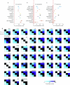
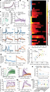
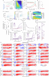
Fig. 1. Widespread representation of sensory evidence, lick preparation and lick execution across the mouse brain during noisy visual change detection.

a, Schematic of the visual change detection task for head-fixed mice. b, Psychometric and reaction-time curves (mean and 95% confidence interval; two-sided Student’s t-test; n = 114 sessions, 15 mice). c, Mean stimulus TF (with 95% confidence interval) preceding early licks during the baseline period. Dashed lines indicate linear mean (1.016 Hz) of baseline stimulus TF. d, Number of units recorded per recording session. e, Brain map of number of units recorded per area across all recording sessions of trained mice. f, Example time series across two trials (a rewarded trial and an early lick trial) of stimulus TF, spike times across simultaneously recorded neurons (two probes), face motion energy (from videography), pupil size and running wheel movement. HPC, hippocampus; TH, thalamus. g, Schematic of single-trial Poisson GLM. Prep., preparation. h, Mean firing rate around early licks (left), and mean response to fast and slow TF pulses during baseline period (right) for an example neuron in MOs and trigeminal motor nucleus (V), together with GLM predicted (on 10% held-out data) mean activity (dashed lines, with 95% confidence interval). Exec., execution; PSTH, peristimulus time histogram. i, Mean (with 95% confidence interval) face motion energy (from videography (Methods)) around early licks, and around fast and slow TF pulses. j, Brain maps with labelled brain regions. See Supplementary Table 2 for definitions of abbreviations. k, Brain maps of percentage of units encoding lick execution (top row), lick preparation (middle row) and stimulus TF fluctuations during the baseline period in the absence of movement (bottom row). l, Percentage of units encoding lick execution, lick preparation and stimulus TF fluctuations during baseline across all brain regions with more than 40 units recorded. Resp., response. See Supplementary Table 1 for number of units recorded in each brain area and Supplementary Table 2 for definitions of brain region abbreviations. *P < 0.05, **P < 0.01, ***P < 0.001. Source Data

Fig. 2. Propagation and widening of fast TF pulse responses across the brain.

a, Schematic of identification of fast (TF pulse > 1 s.d.) and slow (TF pulse < –1 s.d.) TF pulses fluctuating around the mean baseline stimulus TF. b, Single-neuron examples of fast and slow TF pulse responses from selected areas across the brain (mean with 95% confidence interval). FR, firing rate. c, Fast TF pulse responses of all TF-responsive neurons in all brain areas with ten or more TF-responsive units. d, Distribution of response peak times estimated from fast TF pulse responses for each brain area with ten or more TF-responsive units (grey line and circles indicate median peak time per area). e, Comparison of median peak times estimated from fast TF pulse responses (left column) and GLM weights tracking TF fluctuations (GLM TF kernels; see Extended Data Fig. 2 for example kernels; Methods) for each area (right column). f, Distribution of fast TF pulse response half-peak widths (estimated from fast TF pulse responses) for each area with ten or more TF-responsive units (grey line and circles indicate median peak time per area). g, Median fast TF pulse response half-peak widths compared with half-peak widths of the GLM TF kernel. h, Fast TF pulse response peak times across major brain area groupings (median and 95% confidence interval; brain areas in each group are listed in Supplementary Table 1). i, Fast TF pulse response half-peak widths across major brain area groupings (median and 95% confidence interval). Wilcoxon rank sum test. Values of n for each brain area grouping are presented in Supplementary Table 1 and definitions of brain area abbreviations can be found in Supplementary Table 2. NS, not significant. Source Data

Fig. 3. Accumulation of visual evidence as a behavioural strategy and its neural implementation across the brain.

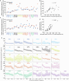
a, Mean stimulus TF preceding early licks in mouse data and outlier-detection agent. Red dashed lines show exponential decay fits. b, Decay time of the exponential fits in a. c, Schematic showing how lick probability is affected by two fast TF pulses that either integrate temporally (black) or act independently (indep.; green). d, Difference between observed early lick probability after two sequential fast TF pulses and the one predicted from their independent effect (Extended Data Fig. 6e–g), normalized by the probability from independent effect, shown as a function of delay between pulses. Data are mean with 95% confidence intervals. e, Responses to a single fast TF pulse (black) or a sequence of two fast pulses separated by 0 s (left) or 0.2 s (right) in example neurons from SCs and MOs. f, Average response to a sequence of two fast TF pulses separated by 0.2 s delay from all TF-responsive neurons in SCs (left) and MOs (right). g, Facilitation of response to the second fast TF pulse as a function of delay between two pulses for TF-responsive units in SCs and MOs. h, Same as g, but for all brain regions with at least ten TF-responsive units. Only time points with 95% confidence interval above zero (bootstrap test) are shown. i, Pearson correlation between second fast TF pulse facilitation and the median half-peak width of response to fast TF pulse across brain regions (P value based on t-statistic). Correlation excludes brain regions without significant facilitation, shown as open circles. j, Average activity of MOs units aligned to TF change onset on hit trials, split by change magnitude. Reaction times (RTs) per magnitude are shown as median (dots) with ranges between 25th and 75th percentiles. k, Same as j, but with the MOs population split into TF-responsive (shades of purple) and TF non-responsive (shades of orange) units. Darker colours correspond to larger change magnitudes. l,m, Mean GLM weights tracking activity after change (change kernels) from SCs (l) and MOs (m) units, derived from activity during change periods. Kernels shown for TF-responsive and non-responsive units, across different change magnitudes. Colour coding as in k. Reaction times shown as in j. a.u., arbitrary units. n, Each dot is the time to 50% of the peak value (ramping time) of the average change kernel across TF-responsive units in early visual areas and frontal cortex (Ctx), shown per change magnitude. o, Scaling of ramping time in activity with change size: each point represents a slope (in seconds per octave) of the linear fit to the dependence shown in m, for each group of brain regions. Bootstrap test. Values of n for each brain region and brain region group are presented in Supplementary Table 1 and definitions of brain area abbreviations can be found in Supplementary Table 2. In all panels, shaded regions or error bars indicate 95% confidence intervals. Source Data

Fig. 4. Representation and integration of visual evidence in association and premotor areas emerges with learning.

a, Schematic of stimulus presentation with random reward delivery used for recordings in untrained mice (Methods). b, Brain maps of unit counts recorded from untrained mice. IRI, inter-reward interval. c, Examples of top two (lowest P value) fast TF-responsive neurons in trained mice (solid lines) or untrained mice (dashed lines) in SCs, VISp, MOs, CP, SIM, DG, MRN and in the orofacial motor nucleus. Norm., normalized. d, Percentage TF-responsive units in all brain areas with more than 40 neurons recorded in both trained and untrained mice. e, Focality index of distribution of TF-responsive units across areas with more than 40 neurons recorded in both untrained and trained mice. In untrained mice, TF-responsive units were confined to a much more limited set of brain regions, compared to trained mice, leading to a significantly higher focality index (n = 24 overlapping brain regions; P < 0.001, bootstrap test (Methods)). Error bars show 95% confidence intervals (Methods). f, Examples of autocorrelation functions from which intrinsic timescales are estimated (that is, τ of decay of autocorrelation function). Error bars are 95% bootstrapped confidence intervals. g, Pearson correlation (P value based on t-statistic) between intrinsic timescales and median half-peak width of responses to a fast TF pulse for all TF-responsive neurons across the brain of trained mice. h, Pearson correlation (P value based on t-statistic) between intrinsic timescales in untrained mice and trained mice. i, Brain maps of intrinsic timescales of trained mice (left) and untrained mice (right). See Supplementary Table 2 for definitions of brain region abbreviations. Source Data

Fig. 5. Preparatory activity is led by TF-responsive subpopulations.

a, Left, mean responses to a fast TF pulse of five example TF-responsive units in MOs (top) and responses to a fast TF pulse for all TF-responsive units in MOs (z-scored firing rate) (bottom). Right, activity of the same neurons aligned to early lick onset. b, Same as a, but for TF-responsive units in SCs. Horizontal black lines indicate windows of activity used to calculate the alignment of population vectors in c. c, Alignment (Pearson correlation; P value based on t-statistic) between responses (baseline subtracted) of TF-responsive MOs or SCs units to a fast TF pulse and their preparatory activity before the early lick. d, Mean alignment of population vectors (correlation in c) for each group of brain regions (bootstrap test). See Supplementary Table 1 for n of each brain region group. e, Fraction of significantly active units (P < 0.01, z-test) as a function of time, shown separately for TF-responsive and TF non-responsive units for six example brain regions. Values of n for each brain region are presented in Supplementary Table 1. f, Fraction of active TF-responsive units (thresholded by lower 95% confidence interval greater than zero, bootstrap test) as a function of time from the hit-lick onset, shown for each brain region. Brain regions are sorted according to the time of the earliest, significantly active fraction (black line; Methods). g, Same as f, but for the TF non-responsive subpopulation. h, Relationship between the onset of preparatory activity in TF-responsive units and their median response duration to a fast TF pulse across brain regions. Pearson correlation and corresponding P value from t-statistic are shown on top. In all panels, shaded regions and error bars indicate 95% confidence interval. See Supplementary Table 2 for definitions of brain region abbreviations. Source Data

Fig. 6. Preparatory activity occupies movement-null subspace, is dominated by TF-responsive subpopulation and is aligned with responses to pulses of sensory evidence.

a, Schematic of two hypothetical ways population activity can transition from movement preparation to execution. Preparatory activity and action execution proceed either along the same mode of activity (single mode hypothesis) or are orthogonal to each other (orthogonal modes hypothesis). Dim., dimension. b, Mean projection of all MOs neuron activities around lick on hit trials onto the first movement dimension, defined by activity in orofacial nuclei in the time window around lick (grey; see Methods). Projection of activity of TF-responsive subpopulation of MOs is shown in blue (Methods; scale on the right); projection from a random (rand.) sample of MOs neurons (grey; matched to number of TF-responsive neurons; scale on the right). c, Projection of MOs activity onto the first movement-null dimension during hit trials. d, Same as b,c, but shown in a state-space formed from first movement and movement-null dimensions. Dots correspond to the state of MOs activity in 10-ms bins. Time relative to lick onset is indicated by colour. e, Relative occupancy of MOs activity in movement versus movement-null subspaces as a function of time (Methods). f, Same as e, but across brain regions (excluding brain regions with poor goodness of fit (R² < 0.8) to activity in orofacial nuclei; Extended Data Fig. 10d). Only time points with relative occupancy significantly different from zero (P < 0.05, bootstrap test) are shown (also for h). Brain regions are sorted according to the earliest latency of significant relative occupancy. Time of peak occupancy in movement-null subspace is shown by the green line. g, Relative contribution of TF-responsive subpopulation to movement-null and movement subspaces. The grey line indicates the value expected from a random sample of neurons from MOs (matched to number of TF-responsive neurons). h, Same as g, but shown across brain regions sorted by latency of significant contribution of TF-responsive subpopulation. Top, fraction of trials with ongoing change epoch. i, Projections of MOs population responses to pulses of sensory evidence onto the first movement-null (top) and movement (bottom) dimensions. j, Cosine of the angle between population response to a fast TF pulse and first movement-null (top) and movement (bottom) dimensions. Data pooled across grouped brain regions (mean ± 95% confidence interval; bootstrap test). k, MOs population responses to pulses of sensory evidence (0–0.5 s after the pulse onset), shown in state-space formed by first movement and movement-null dimensions. Overlaid, MOs preparatory activity (grey) up to 100 ms before hit-lick onset (note the different scale). l, Peak value of projections of MOs responses to a slow or fast TF pulse, or two sequential fast or two sequential slow TF pulses, onto the first movement-null dimension. m, Same as l, but for groups of brain regions (bootstrap test). BG, basal ganglia; CB, cerebellum; FC, frontal cortex; MB, midbrain; Vis.E., visual (early); Vis.H., visual (higher). In all panels, shaded regions or error bars indicate bootstrapped 95% confidence intervals (Methods). Values of n for each brain region or brain region group are presented in Supplementary Table 1 and definitions of brain area abbreviations can be found in Supplementary Table 2. Source Data

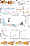
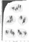
Extended Data Fig. 1. Summary of recordings in trained mice.

a, Number of cells recorded from trained mice in each Allen Brain Atlas designated region. b-f, Locations of all well-isolated and stable units, shown within a 3D rendering of Allen Common Coordinate Framework from five perspectives.

Extended Data Fig. 2. GLM Performance.

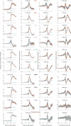
a, Schematic of Poisson GLM. b, Cross-validated model prediction performance of single trial spike counts with full GLM model (r). c, Cross-validated model prediction performance of mean PSTH following fast and slow pulses (r). d, Cross-validated model prediction performance of mean PSTH leading up to an early lick (Lick preparation) (r). e, Cross-validated model prediction performance of mean PSTH after early lick (Lick execution) (r). f, GLM predictions on example neuron recorded in MOs. Top: GLM kernels which the predictions are made from. Bottom: Real vs full GLM predicted vs reduced GLM (without key predictor in model) PSTHs. g, GLM predictions on example neuron recorded in SCs. Top: GLM kernels which the predictions are made from. Bottom: Real vs full GLM predicted vs reduced GLM (without key predictor in model) PSTHs. h, Mean TF kernels across all areas with 10 or more TF-responsive units recorded (for averaging kernels are flipped when needed to always have a positive response). i, Mean lick preparation and lick execution kernels across all areas with 10 or more lick preparation neurons responsive units recorded (for averaging kernels are flipped when needed to always have a positive response).

Extended Data Fig. 3. Encoding of temporal frequency fluctuations, lick preparation and lick execution across brain areas.

a-c, Percentage of units encoding temporal frequency fluctuations during baseline, lick preparation, or lick execution in major area groupings with 95% binomial confidence intervals. a, Percentage lick execution units: All areas: p < 0.001 (Binomial test). b, Percentage lick preparation units: Early visual, Higher visual, Basal ganglia, Frontal cortex, Olfactory nuclei (OLF), Thalamus, Midbrain, Hippocampus, Cerebellum, Lateral hypothalamus (LHA), GRN (Medulla*), Medulla: p < 0.001 (Binomial test), Medulla: p < 0.01 (Binomial test). c, Percentage TF Responsive units: Early visual, Higher visual, Basal ganglia, Frontal cortex, Thalamus, Midbrain, Hippocampus, Cerebellum, GRN (Medulla*): p < 0.001 (Binomial test), Olfactory nuclei (OLF), Lateral hypothalamus (LHA), and Medulla: p > 0.05 (Binomial test). Error bars in panels a-c are 95% binomial confidence intervals. Red areas designate chance level. See Supplementary Table 1 for n of each brain area grouping. d, Percentage overlap of encoding (estimated from GLM) of TF, lick preparation, and lick execution, in all areas with more than 40 units recorded. y-axis is the source population (i.e., all TF responsive neurons, all lick preparation neurons, or all lick execution neurons).

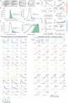
Extended Data Fig. 4. Responses of TF responsive neurons across the brain to fast or slow TF pulses and early licks.

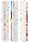
Activity (z-scored) of individual neurons around fast TF pulses (left), slow TF pulses (middle) and early licks (right) for all TF responsive units from all areas with 10 or more TF responsive units recorded. Major subdivisions of the brain grouped by colour. Each line represents one neuron.

Extended Data Fig. 5. Properties of responses to a single fast TF pulse from PSTHs and GLM + Relative facilitation by the second fast TF pulse as a function of delay from the first one.

a-d, Comparison of peak time and response width of PSTHs following a fast TF pulse vs GLM TF kernels. a, Median peak time of response to a fast TF pulse estimated from PSTH (red) and median peak time of GLM TF kernel (blue), shown for each brain region. b, Correlation across brain regions between median peak time estimated from PSTH and median peak time of GLM TF kernel. c-d, Same as a-b, but for fast TF pulse response half-peak width. e, Relative facilitation by the second fast TF pulse, normalized by the response to a single fast TF pulse, shown as a function of delay between two fast TF pulses for each brain region with at least 10 TF responsive units (mean and 95% confidence intervals, bootstrap test (see Methods)). Values close to zero imply no facilitation (same size of response to the second fast TF pulse as to the first one), while values close to 100% imply doubling of the response size.

Extended Data Fig. 6. Effect of magnitude and timing of TF pulses on probability of early licks.

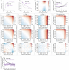
a, Mean performance (psychometric curves) for mice data (dashed black line, n = 15 mice) and outlier detection agent (purple). b, Mean reaction times per change magnitude for outlier detection agent (purple) and mice data (dashed black line, n = 15 mice). Error bars indicate 95% confidence intervals across 4000 synthetic datasets of the model (see Methods). c, Conditional probability of early lick at a specific time after a TF pulse of given magnitude. Here and later early lick probability is shown relative to the probability at the mean baseline TF (1 Hz). d, Probability of early lick after a TF pulse of given magnitude (here and later cumulatively within [0.2, 1] s window). Mice data is shown in black, outlier detection agent – in purple (mean and non-parametric 95% confidence intervals, see Methods). e, Upper panel: probability of early lick after two sequential TF pulses of given magnitudes; middle panel: expected effect if both pulses influence early lick probability independently; lower panel: difference from the independent effect of TF pulses. f-g, The same format as in e, but for two TF pulses with 100 ms or 500 ms delay between them. h, The same format as in c, but shown for data generated by the outlier detection agent (for two sequential TF pulses). i, Difference in probability of early lick relative to the independent effect after a sequence of two fast TF pulses (top right corner in lower panels e-g), normalized by the expected probability from the effect of independent pulses and shown as a function of delay between fast TF pulses. The results of the same analysis applied to the outlier detection agent data are shown in purple (mean and non-parametric 95% confidence intervals, see Methods).

Extended Data Fig. 7. A simple two parameter leaky integrator model supports behavioural evidence integration + GLM change kernels across individual areas and large area groupings.

a, Schematic of the leaky-integrator model. b, Parameter search grid identifying which values the integration time and threshold best predicts early licks (i.e., correct predictions of early lick times (on single trials). c, Lick triggered stimulus average of early licks detected by the leaky integrator model, and early licks not detected by the model. d, Best-fit integration decay time of leaky-integrator model, shown per mouse (black dots) and mean across animals (n = 15 mice, error bar is 95% confidence intervals). ***p < 0.001, two sided t-test. e, Relationship between real reaction time and predicted reaction time from leaky integrator model (tau: 0.25 s) for change size 1.25 Hz of example mouse 12. Correlation is calculated across all reaction times. f, Same as f but for change size 1.35 Hz. g, Correlation between observed and predicted reaction times during the change period for outlier detection agent (no integration, top) and leaky-integrator model (bottom). Threshold parameters corresponding to best-fit were used for each model. The colour along each row corresponds to the correlation value between predicted hit lick reaction times and actual hit lick reaction times on trials with that change magnitude, conditioned by the maximum RT included for this analysis (cutoff time). h, Summary of panel g with results shown per mouse and RT combined across all change magnitudes (RT cutoff equal to 1 second from change onset). n = 15 mice, ***p < 0.001, two sided t-test. i, Mean decision value (integrated TF) after filtering stimulus though a leaky integrator model with a tau of 0.25 s. j, Mean reaction time curve for leaky integrator model. k, Example trials around change onset when model has no integration. Note the similarity to change kernels of TF responsive units in the SCs in Fig 3l. l, Example trials around change onset when model has leaky integration (0.25 s tau). Note the similarity to change kernels of to TF responsive units in the MOs in Fig 3l. m, Leaky evidence integration smooths and denoises the noisy sensory input so that the signal-to-noise ratio (S/σ) is considerably larger 0.5 s after change onset, compared to no integration–- making detection of noisy changes easier. n, Change size specific GLM change kernels for all areas recorded with 10 or more TF responsive units. o, Change size specific change kernels for major area groupings. Dotted line indicates the 50% response crossing for each change size.

Extended Data Fig. 8. Intrinsic vs learned TF pulse response properties.

a, Percentage of units encoding temporal frequency fluctuation during baseline in major area groupings with 95% binomial confidences in untrained and trained mice. Stars designate significance of difference (binomial test) in fractions between naïve and trained mice: n.s.: Not significant, ** p < 0.01, ***p < 0.001, binomial tests. Error bars are 95% binomial confidence intervals. OLF: Olfactory nuclei, Ctx: Cortex. See Supplementary Table 1 for n of each brain area grouping. b, Intrinsic timescales (tau) estimated for each TF responsive unit across the brain vs the TF response width for those units. Intrinsic times scales do not correlate with TF response width at a single cell level (p > 0.05, Pearson correlation, p-value is based on t-statistic). c, Same as in a but with units divided into major area groups. No area group has significant correlation between intrinsic times scales and TF response width at a single cell level (p > 0.05, Pearson correlation, p-value is based on t-statistic). d, Same as Fig. 4g, but here areal intrinsic time scale is extracted from TF responsive units only. In agreement with Fig. 4g, there is no correlation (Pearson correlation, p-value is based on t-statistic) between areal intrinsic timescales and median TF response width. e, intrinsic timescales of TF responsive units are similar to the intrinsic timescales as areas as a whole (Pearson correlation, p-value is based on t-statistic).

Extended Data Fig. 9. Differences in timing of preparatory activity between TF responsive and TF non-responsive populations.

a, Fraction of active units (combined across TF responsive and TF non-responsive units) as a function of time from the hit lick onset, shown across brain regions. Shades of red indicate a higher level of activity. Time points with lower 95% confidence interval (bootstrap test, see Methods) smaller than zero are shown as white. Brain regions are sorted according to the time of the first significant activation (blue line, see Methods). Black line shows the time of first significant activation using the same criterion as for Fig. 5f,g. b, Difference in onsets of preparatory activity across TF responsive and TF non-responsive subpopulations. Positive values indicate that TF responsive subpopulation has an earlier preparatory activity. Significant differences from zero are indicated by number of stars and area shaded in grey indicates 95% confidence intervals (bootstrap test, see Methods). * p < 0.05, ** p < 0.01, ***p < 0.001. c, Difference in levels of activity between TF responsive and TF non-responsive subpopulations within each brain region. Shades of red indicate a higher level of activity across TF responsive subpopulation. Time points with non-significant differences (p ≥ 0.05, bootstrap test) in activity are shown as white. Brain regions are sorted according to the latency of the first significant difference in activation between TF responsive and non-responsive subpopulations (black line). d, Pearson correlation (p-value is based on t-statistic) across brain regions between the latency of the first significant difference in activation between TF responsive and TF non-responsive subpopulations and the median half-peak width of response to a fast pulse.

Extended Data Fig. 10. Definition of movement and movement-null subspaces.

a, Cross-validated cumulative R-squared coefficient of activity aligned to the hit lick onset shown across first six principal components for each brain region. Brain regions are sorted by the maximum cumulative R-squared value. b, Projections onto first four principal components of orofacial nuclei activity aligned to the hit lick onset. Projections on the first two principal components define the temporal profiles of activity within the two-dimensional movement subspace. The amount of cross-validated variance (average across draws) captured by each principal component is indicated on each panel. c, Projections of MOs activity (orange) aligned to the hit lick onset onto two movement (top) and two movement-null (bottom) dimensions. Projections of orofacial nuclei activity onto movement dimensions are shown in brown. d, Average cross-validated R-squared coefficient of mapping onto the movement subspace, with brain regions ordered from the best to worst mapping accuracy. The minimal value of R-squared coefficient for a brain region to be considered to have a good mapping onto a movement subspace is shown as a dashed red line (0.8). In all panels shaded regions indicate non-parametric 95% confidence intervals (see Methods).

Extended Data Fig. 11. Occupancy of movement and movement-null subspaces and contribution of TF-responsive subpopulation within them.

a, Peak-normalized occupancy of movement subspace as a function of time for each brain region, relative to the hit lick onset time. Here and on panels b,c the order of brain regions is the same as on Fig. 6f. b, Peak-normalized occupancy of movement-null subspace as a function of time for each brain region. c, Average time of the peak occupancy within the movement-null subspace (green line), shown for each brain region. Shading indicates 95% confidence intervals. d, Distribution of loadings values along the first movement-null dimension that correspond to TF responsive (blue) and TF non-responsive (black) units in MOs. e, Minus log of p-value (blue line) for a paired 2-sided t-test between absolute values of loadings along the first movement-null dimension that correspond to TF responsive and TF non-responsive units. Dashed grey line indicates p = 0.05 level. c, Related to Fig. 6h. Comparison (Wilcoxon signed-rank test) of half-peak width of response to fast TF pulse between brain regions that had a disproportionate contribution of TF responsive subpopulation to preparatory activity in movement-null subspace (left bar, n = 16 brain regions) and the rest of brain regions (right bar, n = 12 brain regions). Bars indicate the mean across brain regions, error bars – 95% confidence intervals of the mean (bootstrap test, 2000 times). f, Relative contribution of TF responsive subpopulation within the movement subspace as a function of time for each brain region. Brain regions are shown in the same order as on Fig. 6h.

Extended Data Fig. 12. Alignment and scaling of TF pulse response projections on movement and movement-null dimensions.

a, Cosine of the angle between population response to a fast TF pulse and movement or movement-null dimensions. Values that are significantly different from zero (p < 0.05, 2-sided bootstrap test) are indicated by the black outline. b, Peak value of projections onto the first movement-null dimension of responses to a slow, fast, two sequential slow, and two sequential fast TF pulses. Results are shown for each brain region as the mean and 95% confidence intervals over 2000 cross-validations (see Methods). See Supplementary Table 1 for number of neurons in each brain region. Number of starts indicates a 2-sided bootstrap test p-value of difference from zero for population response to a single fast or slow TF pulse, or a significance of a difference between responses to one or two sequential TF pulses. * p < 0.05, ** p < 0.01, ***p < 0.001. Non-significant effects are not indicated.

Extended Data Fig. 13. Breakdown of projections on main principal components by contributions from TF responsive and TF-nonresponsive units.

Each row shows projections on four main principal components of population activity within a given brain region aligned to the hit lick onset (same as on Fig. 6). The time course of each projection (black) was decomposed into a sum of contributions from TF responsive (blue) and TF non-responsive (red) units. Grey line indicates projection expected from a random sample of the same size as there were TF responsive units, taken randomly (with replacement) from the full population. Data is shown as mean and 95% confidence intervals across 2000 cross-validations (see Methods). The amount of cross-validated variance captured by each principal component is indicated on top of each panel.

References

1. Gold, J. I. & Shadlen, M. N. The neural basis of decision making. Annu. Rev. Neurosci.30, 535–574 (2007). - PubMed
1. Hanks, T. D. & Summerfield, C. Perceptual decision making in rodents, monkeys, and humans. Neuron93, 15–31 (2017). - PubMed
1. Steinmetz, N. A., Zatka-Haas, P., Carandini, M. & Harris, K. D. Distributed coding of choice, action and engagement across the mouse brain. Nature576, 266–273 (2019). - PMC - PubMed
1. Chen, S. et al. Brain-wide neural activity underlying memory-guided movement. Cell187, 676–691 (2024). - PMC - PubMed
1. Allen, W. E. et al. Thirst regulates motivated behavior through modulation of brainwide neural population dynamics. Science364, 253 (2019). - PMC - PubMed
LinkOut - more resources