Landau-phonon polaritons in Dirac heterostructures

Abstract

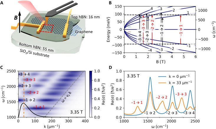
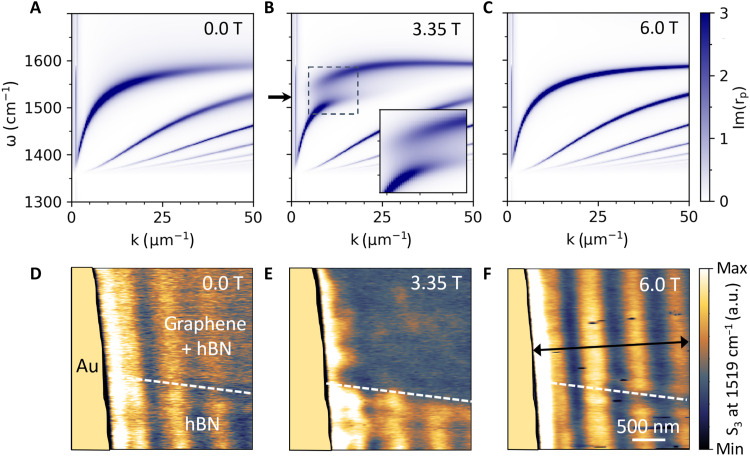
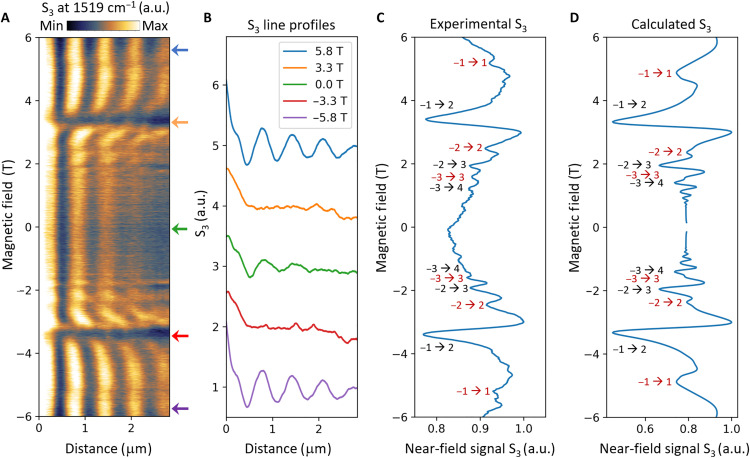
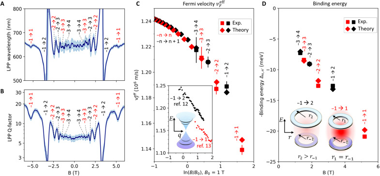
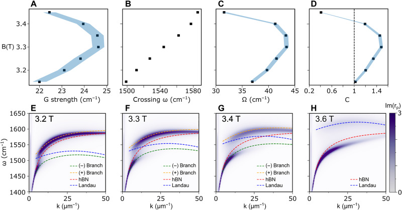
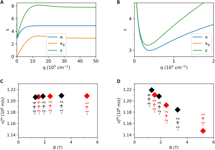
Polaritons are light-matter quasiparticles that govern the optical response of quantum materials at the nanoscale, enabling on-chip communication and local sensing. Here, we report Landau-phonon polaritons (LPPs) in magnetized charge-neutral graphene encapsulated in hexagonal boron nitride (hBN). These quasiparticles emerge from the interaction of Dirac magnetoexciton modes in graphene with the hyperbolic phonon polariton modes in hBN. Using infrared magneto-nanoscopy, we reveal the ability to completely halt the LPP propagation in real space at quantized magnetic fields, defying the conventional optical selection rules. The LPP-based nanoscopy also tells apart two fundamental many-body phenomena: the Fermi velocity renormalization and field-dependent magnetoexciton binding energies. Our results highlight the potential of magnetically tuned Dirac heterostructures for precise nanoscale control and sensing of light-matter interaction.

Fig. 1.. High-momentum magneto-optics of graphene.

(A) Schematics of our sample and m-SNOM setup. Gold contacts enable transport measurements and gating of graphene and also serve as polariton launchers. (B) LL energy as a function of magnetic field B and LL index n = 0, ±1, …, ±4. Black (red) arrows mark −n → n ± 1 and −n → n inter-LL transitions (ILTs) for a photon energy of ℏω = 188 meV (1519 cm⁻¹). (C) Analytically calculated real part of the graphene conductivity (43) at B = 3.35 T as a function of frequency ω and in-plane momentum k calculated using Fermi velocity v_F = 1.19 × 10⁶ m/s and damping γ = 24.3 cm⁻¹. The relevant −n → n ± 1 (−n → n) ILTs are labeled in black (red). The black bell-shaped curve illustrates the momenta accessible via m-SNOM (14), which peak at around k = 1/r_tip = 33 μm⁻¹ as marked by the vertical dashed line. (D) The line cuts at momenta k = 0 and k = 33 μm⁻¹ extracted from (C).

Fig. 2.. Hybridization of hBN phonon polaritons with graphene Landau polaritons, resulting in LPPs.

(A to C) Calculated LPP dispersion at magnetic fields of 0.0, 3.35, and 6.0 T, respectively. The false color represents Im r_p(k, ω), the analytically calculated imaginary part of the reflection coefficient for p-polarized light. Graphene is assumed to be charge neutral with a constant LL broadening (33) γ = 24.3 cm⁻¹ and Fermi velocity v_F = 1.19 × 10⁶ m/s, the latter being the value extracted from Fig. 4C. Inset in (B): An enlarged view of the region exhibiting strong coupling and an avoided crossing between the Landau and the hBN phonon polaritons; the arrow marks ω = 1519 cm⁻¹ corresponding to the data in (D) to (F). (D to F) Nano-imaging data collected from the region marked by the red rectangle in Fig. 1A at T = 154 K and B = 0.0, 3.35, and 6.0 T, respectively. The near-field signal S₃ (demodulated at the third harmonic of the tip frequency; refer to Materials and Methods) shows relative differences between regions with and without graphene that strongly depend on the magnetic field. The enhanced signal-to-noise ratio in (E) and (F), compared to (D), is due to a slightly longer integration time. We also note that the mechanical stability of our system is slightly better at higher magnetic fields. The double-headed arrow in (F) marks the location of the line scan analyzed further in Fig. 3. a.u., arbitrary unit.

Fig. 3.. Magnetic-field dependence of the polariton dispersion.

(A) Near-field signal S₃ acquired via a repeated line scan while sweeping the magnetic field from −6.0 to 6.0 T at a rate of 0.4 mT/s; measurement was taken at ω = 1519 cm⁻¹ and T = 154 K. The direction of this line scan was perpendicular to the gold contact to the left, which served as a polariton launcher; see Figs. 1A and 2F. (B) Line profiles extracted from (A) at magnetic fields B = 0.0, ±3.3, and ±5.8 T. (C) The near-field signal in (A) averaged over the distance. Minima of the averaged signal are assigned to the ILTs shown by the labels. The assignment is based on the calculation shown in (D). (D) Calculated near-field signal (Materials and Methods) as a function of magnetic field. Parameter values are chosen to be the same as in Figs. 1 (C and D) and 2 (A to C).

Fig. 4.. Magnetic-field dependence of LPP properties and Fermi velocity renormalization.

(A) Polariton wavelength λ_P and (B) polariton quality factor Q = Re k/ Im k as a function of the magnetic field B. Solid lines show experimental values extracted from Fig. 2; shaded regions show the SD of the measurement. (C) Effective Fermi velocity ${\mathrm{v}}_{\mathrm{F}}^{\text{eff}}$ as a function of the logarithmic magnetic field ln(B) derived for different ILTs (see section Many-body effects): Squares show experimental values derived from (B). Diamonds represent calculated values of ${\mathrm{v}}_{\mathrm{F}}^{\text{eff}}$ (see Materials and Methods) (37). We observe a nonlogarithmic trend. Inset: The red (black) points show ${\mathrm{v}}_{\mathrm{F}}^{\text{eff}}$ for the −1 → 1 (−1 → 2) ILT measured via Raman spectroscopy (34) [far-field infrared spectroscopy (33)]. The tapering shape of the Dirac cone illustrates the Fermi velocity renormalization (33, 34, 40), resulting in a logarithmic B dependence of the far-field data (33, 34). (D) Squares and diamonds show the exciton binding energy ${\mathrm{\Delta }}_{\mathrm{n}\mathrm{n}\prime }$ of the Landau polaritons derived from the experiment and theory, respectively. The exciton binding energy is larger for the ILTs with $n\prime$ = −n compared to those with $n\prime$ = −(n ± 1) and generally increases with magnetic field. Inset: The dependence of the exciton binding energy on the magnetic field and type of the ILT can be explained within a semiclassical model where quantized electronic orbitals of the LLs are shaped as narrow rings of radius ${\mathrm{r}}_{\mathrm{j}}={\mathrm{l}}_{\mathrm{B}}\sqrt{2\left|j\right|}$, j = n, or $n\prime$. The magnetoexciton binding energy ${\mathrm{\Delta }}_{\mathrm{n}\mathrm{n}\prime }$ (see text) is given by the Coulomb attraction energy of these rings. For a fixed n, this binding energy is the largest when the ring radii are equal, at $n\prime$ = −n.

Fig. 5.. Gate dependence of the −1➔ 2 graphene LPP at B = 3.3 T.

(A) Near-field signal acquired via a repeated scan of the same line as in Fig. 3A while sweeping the gate voltage and, thus, the filling factor from ν = 0 to 19; measurements were done at ω = 1519 cm⁻¹, and T = 154 K. (B) Line profiles extracted from (A) at four different filling factors of ν = 0, 5, 10, and 15, respectively. (C) Polariton wavelength λ_P and (D) polariton Q factor as a function of ν and charge carrier concentration N at 3.3 T; the shaded regions show the SD of the measurement.

Fig. 6.. Frequency dependence of the gate dependence at B = 3.3 T.

Near-field signal acquired via a repeated scan of approximately the same line as in Fig. 3A while sweeping the back gate voltage from 0 to −50 V. The charge neutrality point (CNP) of graphene for these scans is found approximately in the middle of the scans, i.e., around −25 V. To investigate the dependence on the photon energy, the scans were performed at different frequencies, from left to right: ω = 1498,1509,1519,1529,1537,1547 cm⁻¹. The measurements were done at temperature T = 76 K. Scale bar, 1 μm.

Fig. 7.. Extraction of oscillator parameters from polariton dispersions.

(A) Im r_p at B = 6 T from the main text (Fig. 2C). The red-shaded region indicates the area excluded by the window function. The white solid line is the phonon polariton dispersion extracted from fitting. (B) Line profiles from (A) extracted for different momenta values (black lines). The fitted curve is represented as dashed lines. (C) hBN phonon polaritons damping and oscillator strength extracted from fitting. (D) Im r_p simulated for graphene on SiO₂ (thickness, 285 nm) at B = 3.35 T. The black solid line represents the dispersion extracted from fitting. (E) Extracted Landau polariton resonance as a function of magnetic field and momenta. The white dashed lines represent isofrequencies. (F) Landau polariton damping and oscillator strength from fitting.

Fig. 8.. Determination of coupling strength from hybrid modes.

(A and D) Extracted dispersion of lower (green) and upper (yellow) branches for (A) B = 3.15 T and (D) B = 3.4 T. The simulated Im r_p and the dispersion of the uncoupled modes are shown for reference. Dependence of 2Δω_±(q) on (B and E) the real part and (C and F) the imaginary part of H(k) for B = 3.15 T and B = 3.4 T.

Fig. 9.. Coupling strength analysis and model validation across varying magnetic fields.

(A) Coupling strength as a function of the magnetic field, extracted via fitting. (B) Extracted spectral position where the hBN phonon polariton and Landau polariton dispersion cross. (C) Branch separation Ω at the crossing point. (D) Criterion C for strong coupling. The blue-shaded areas represent the uncertainty of the presented variables, assuming straight connections between the data points as a guide to the eye. (E to H) Calculated branch dispersion based on the uncoupled modes and the extracted coupling strength for (E) B = 3.2 T, (F) B = 3.3 T, and (G) B = 3.4 T. For (H) B = 3.6 T, we only show the hBN phonon polariton and the Landau polariton dispersions. The Im(r_p) is presented on the background to show the expected dispersion from the simulation.

Fig. 10.. Calculation of the Fermi velocities and many-body effects.

(A and B) Effective dielectric function for electrons in graphene. Functions κ(q), κ_g(q), and ϵ(q) defined by Eq. 19 (A to C) for B = 3.35 T. (B) shows a magnification of the small dip at low q that is observed for κ_g(q) and ϵ(q). (C) Renormalized Fermi velocities given by Eq. 26. (D) Effective Fermi velocities defined by Eq. 17 that include excitonic corrections.

References

1. Low T., Chaves A., Caldwell J. D., Kumar A., Fang N. X., Avouris P., Heinz T. F., Guinea F., Martin-Moreno L., Koppens F., Polaritons in layered two-dimensional materials. Nat. Mater. 16, 182–194 (2017). - PubMed
1. Zhang Q., Hu G., Ma W., Li P., Krasnok A., Hillenbrand R., Alù A., Qiu C.-W., Interface nano-optics with van der Waals polaritons. Nature 597, 187–195 (2021). - PubMed
1. Basov D. N., Fogler M. M., Garcia de Abajo F. J., Polaritons in van der Waals materials. Science 354, aag1992 (2016). - PubMed
1. Dirnberger F., Quan J., Bushati R., Diederich G. M., Florian M., Klein J., Mosina K., Sofer Z., Xu X., Kamra A., García-Vidal F. J., Alù A., Menon V. M., Magneto-optics in a van der Waals magnet tuned by self-hybridized polaritons. Nature 620, 533–537 (2023). - PubMed
1. Basov D. N., Asenjo-Garcia A., Schuck P. J., Zhu X., Rubio A., Polariton panorama. Nanophotonics 10, 549–577 (2020).
LinkOut - more resources