A next-generation, histological atlas of the human brain and its application to automated brain MRI segmentation

Abstract

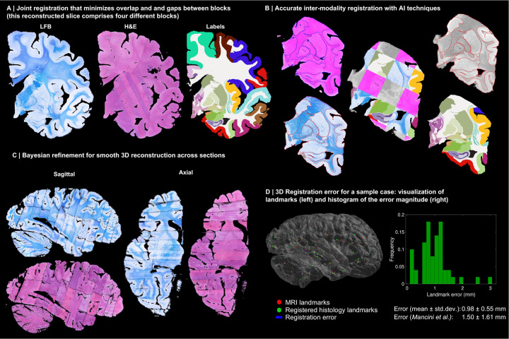
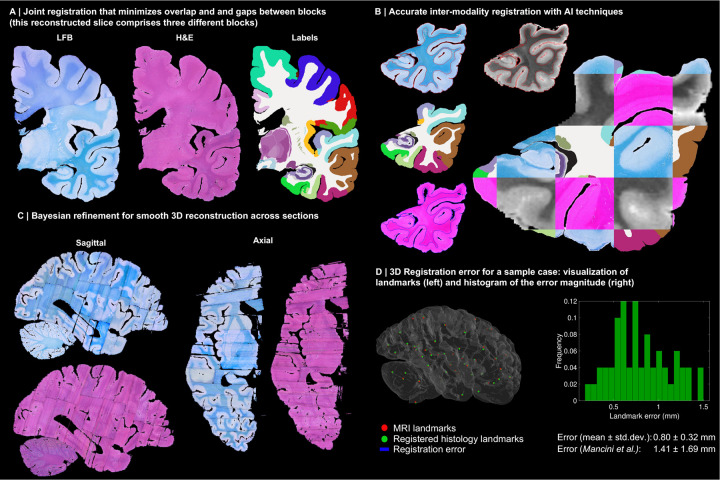
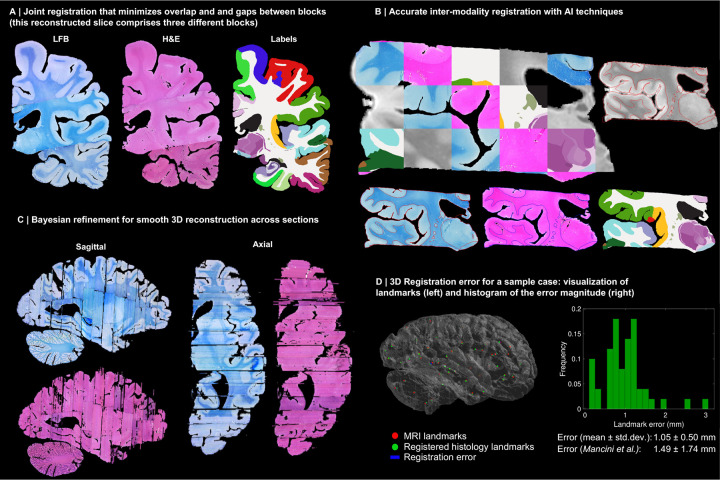
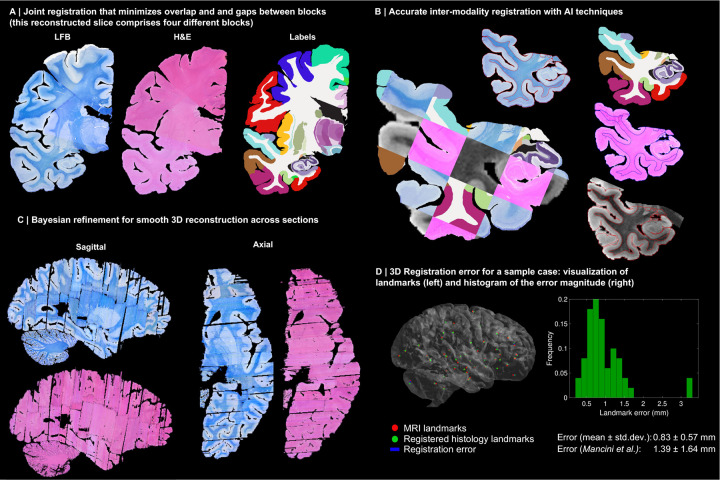
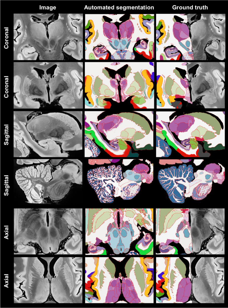
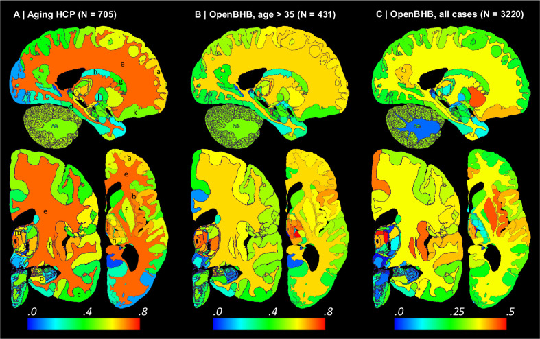
Magnetic resonance imaging (MRI) is the standard tool to image the human brain in vivo. In this domain, digital brain atlases are essential for subject-specific segmentation of anatomical regions of interest (ROIs) and spatial comparison of neuroanatomy from different subjects in a common coordinate frame. High-resolution, digital atlases derived from histology (e.g., Allen atlas [7], BigBrain [13], Julich [15]), are currently the state of the art and provide exquisite 3D cytoarchitectural maps, but lack probabilistic labels throughout the whole brain. Here we present NextBrain, a next-generation probabilistic atlas of human brain anatomy built from serial 3D histology and corresponding highly granular delineations of five whole brain hemispheres. We developed AI techniques to align and reconstruct ~10,000 histological sections into coherent 3D volumes with joint geometric constraints (no overlap or gaps between sections), as well as to semi-automatically trace the boundaries of 333 distinct anatomical ROIs on all these sections. Comprehensive delineation on multiple cases enabled us to build the first probabilistic histological atlas of the whole human brain. Further, we created a companion Bayesian tool for automated segmentation of the 333 ROIs in any in vivo or ex vivo brain MRI scan using the NextBrain atlas. We showcase two applications of the atlas: automated segmentation of ultra-high-resolution ex vivo MRI and volumetric analysis of Alzheimer's disease and healthy brain ageing based on ~4,000 publicly available in vivo MRI scans. We publicly release: the raw and aligned data (including an online visualisation tool); the probabilistic atlas; the segmentation tool; and ground truth delineations for a 100 μm isotropic ex vivo hemisphere (that we use for quantitative evaluation of our segmentation method in this paper). By enabling researchers worldwide to analyse brain MRI scans at a superior level of granularity without manual effort or highly specific neuroanatomical knowledge, NextBrain holds promise to increase the specificity of MRI findings and ultimately accelerate our quest to understand the human brain in health and disease.

Extended Data Fig. 1:

3D reconstruction of Case 2. The visualisation follows the same convention as in Figure 3: (A) Coronal slice of the 3D reconstruction. (B) Registered MRI, LFB, and H&E histology of a block, with tissue boundaries (traced on LFB) overlaid. (C) Orthogonal view of reconstruction, which is smooth and avoids gaps and overlaps. (D) Visualization of 3D landmark registration error (left); histogram of its error (right); and mean ± standard deviation (bottom), compared with our previous pipeline (Mancini et al. [6]).

Extended Data Fig. 2:

3D reconstruction of Case 3. The visualisation follows the same convention as in Figure 3: (A) Coronal slice of the 3D reconstruction. (B) Registered MRI, LFB, and H&E histology of a block, with tissue boundaries (traced on LFB) overlaid. (C) Orthogonal view of reconstruction, which is smooth and avoids gaps and overlaps. (D) Visualization of 3D landmark registration error (left); histogram of its error (right); and mean ± standard deviation (bottom), compared with our previous pipeline (Mancini et al. [6]).

Extended Data Fig. 3:

3D reconstruction of Case 4. The visualisation follows the same convention as in Figure 3: (A) Coronal slice of the 3D reconstruction. (B) Registered MRI, LFB, and H&E histology of a block, with tissue boundaries (traced on LFB) overlaid. (C) Orthogonal view of reconstruction, which is smooth and avoids gaps and overlaps. (D) Visualization of 3D landmark registration error (left); histogram of its error (right); and mean ± standard deviation (bottom), compared with our previous pipeline (Mancini et al. [6]).

Extended Data Fig. 4:

3D reconstruction of Case 5. The visualisation follows the same convention as in Figure 3: (A) Coronal slice of the 3D reconstruction. (B) Registered MRI, LFB, and H&E histology of a block, with tissue boundaries (traced on LFB) overlaid. (C) Orthogonal view of reconstruction, which is smooth and avoids gaps and overlaps. (D) Visualization of 3D landmark registration error (left); histogram of its error (right); and mean ± standard deviation (bottom), compared with our previous pipeline (Mancini et al. [6]).

Extended Data Fig. 5:

Sagittal, coronal, and axial slices of the continuous maps of the 3D landmark registration error. The maps are computed from the discrete landmarks (displayed in Fig. 3D and Extended Data Figs. 1–4D) using Gaussian kernel regression with σ = 10 mm. There is no clear spatial pattern for the anatomical distribution of the error across subjects.

Extended Data Fig. 6:

Box plots of the Dice scores for 11 representative ROIs computed on the OpenBHB dataset (3,330 subjects), using the Allen MNI template and NextBrain, with FreeSurfer segmentations as reference. The scores are computed at the whole regions level, i.e., the level of granularity at which FreeSurfer segments. On each box, the central mark indicates the median, the edges of the box indicate the 25^th and 75^th percentiles, the whiskers extend to the most extreme data points not considered outliers, and the outliers are plotted individually as ‘+’. The abbreviations for the regions are: WM = white matter of the cerebrum, CT = cortex of the cerebrum, CWM = cerebellar white matter, CCT = cerebellar cortex, TH = thalamus, CA = caudate, PU = putamen, PA = pallidum, BS = brainstem, HP = hippocampus, AM = amygdala.

Extended Data Fig. 7:

Absolute value of Spearman correlation for ROI volumes vs age derived from in vivo MRI scans (additional slices). The visualisation follows the same convention as in Figure 5: (A) Ageing HCP dataset. (B) OpenBHB dataset, restricted to ages over 35. (C) Full OpenBHB dataset.

Extended Data Fig. 8:

Aging trajectories for select ROIs in HCP dataset, showing differential pattens in subregions of brain structures (thalamus, hippocampus, cortex, etc). The red dots correspond to the ROI volumes of individual subjects, corrected by intracranial volume (by division) and sex (by regression). The blue lines represent the maximum likehood fit of a Laplace distribution with location and scale parameters parametrised by a B-spline with four control points (equally space between 30 and 95 years). The continuous blue line represents the location, whereas the dashed lines represent the 95% confidence interval (equal to three times the scale parameter in either direction). Volumes of contralateral structures are averaged across left and right.

Fig. 1:

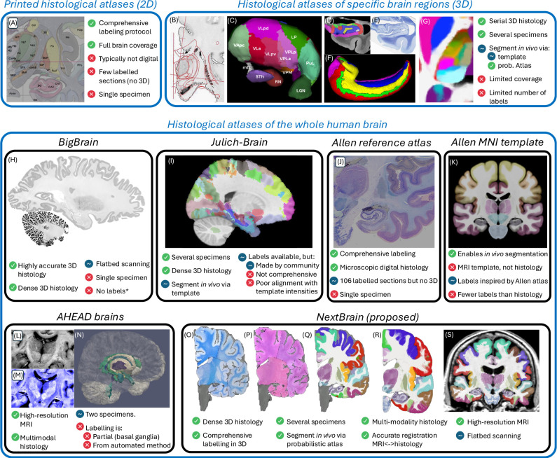
NextBrain in the context of histological atlases, with advantages (), disadvantages (), and neutral points. (). (A) Printed atlas [1] with a sparse set of manually traced sections [1]. (B-G) Histological atlases of specific ROIs with limited coverage: (B) Manually traced section of basal ganglia [8]; (C) 3D rendering of deterministic thalamic atlas [11]; (D-F) Traced MRI slice, histological section, and 3D rendering of hippocampal atlas [12]; and (G) Slice of our probabilistic atlas of the thalamus [14]. (H-N) Histological atlases of the whole human brain: (H) 3D reconstructed slice of BigBrain [13]; (I) Slice of Julich-Brain labels on MNI template; (J) Labelled histological section of the Allen reference brain [7]; (K) Labelling of MNI template with protocol inspired by (J); and (L-N) MRI, histology, and 3D rendering of AHEAD brains [22]. (O-S) Our new atlas NextBrain includes dense 3D histology (O-P) and comprehensive manual labels (Q) of five specimens, enabling the construction of a probabilistic atlas (R) that can be combined with Bayesian techniques to automatically label 333 ROIs in in vivo MRI scans (S).

Fig 2:

NextBrain workflow. (A) Photograph of formalin-fixed hemisphere. (B) High-resolution (400 μm) ex vivo MRI scan, FreeSurfer segmentation, and extracted pial surface (parcellated with FreeSurfer). (C) Tissue slabs and blocks, before and after paraffin embedding. (D) Section stained with H&E and LFB. (E) Semi-automated labelling of 333 ROIs on sections using an Al method [5]. (F) Initialization of affine alignment of tissue blocks using a custom registration algorithm that minimises overlap and gaps between blocks. (G) Refinement of registration with histology and nonlinear transform, using a combination of Al and Bayesian techniques [9,10]. (H) Orthogonal slices of 3D probabilistic atlas. (I) Automated Bayesian segmentation of an in vivo scan into 333 ROIs using the atlas.

Fig. 3:

3D reconstruction of Case 1. (A) Coronal slice of 3D reconstruction; boundaries between blocks are noticeable from uneven staining. (B) Registered MRI, LFB, and H&E histology of a block, with tissue boundaries (traced on LFB) overlaid. (C) Orthogonal view of reconstruction, which is smooth thanks to the Bayesian refinement, and avoids gaps and overlaps thanks to the regulariser. (D) Visualization of 3D landmark registration error (left); histogram of its magnitude (right); and mean ± standard deviation (bottom), compared with our previous pipeline [6]. See Extended Data for results on the other cases. The average landmark error across all cases is 0.99mm (vs 1.45 for [6]).

Fig. 4:

NextBrain probabilistic atlas. (A) Portions of the NextBrain probabilistic atlas (which has 333 ROIs), the SAMSEG atlas in FreeSurfer [2] (13 ROIs), and the manual labels of MNI based on the Allen atlas [7] (138 ROIs). (B) Close-up of three orthogonal slices of NextBrain. The colour coding follows the convention of the Allen atlas [7], where the hue indicates the structure (e.g., purple is thalamus, violet is hippocampus, green is amygdala) and the saturation is proportional to neuronal density. The colour of each voxel is a weighted sum of the colour corresponding to the ROIs, weighted by the corresponding probabilities at that voxel. The red lines separate ROIs based on the most probable label at each voxel, thus highlighting boundaries between ROIs of similar colour; we note that the jagged boundaries are a common discretization artefact of probabilistic atlases in regions where two or more labels mix continuously, e.g., the two layers of the cerebellar cortex.

Fig. 5:

Automated Bayesian segmentation of publicly available ultra-high resolution ex vivo brain MRI [3] using the simplified version of NextBrain, and comparison with ground truth (only available for right hemisphere). We show two coronal, sagittal, and axial slices. The MRI was resampled to 200 μm isotropic resolution for processing. As in previous figures, the segmentation uses the Allen colour map [7] with boundaries overlaid in red. We note that the manual segmentation uses a coarser labelling protocol.

Fig. 6:

Absolute value of Spearman correlation for ROI volumes vs age derived from in vivo MRI scans: (A) Ageing HCP dataset (image resolution: .8mm isotropic; age range: 36–90 years; mean age: 59.6 years); please see main text for meaning of markers (letters). (B) OpenBHB dataset [4], restricted to subjects with ages over 35 years to match Ageing HCP (resolution 1 mm isotropic; age range: 36–86 years; mean age: 57.9 years). (C) Full OpenBHB dataset (age range: 6–86 years, mean age: 25.2 years); please note the different scale of the colour bar. The ROI volumes are corrected by intracranial volume (by division) and sex (by regression). Further slices are shown in Extended Data Fig. 6.

References

1. Mai J. K., Majtanik M. & Paxinos G. Atlas of the human brain. (Academic Press, 2015).
1. Puonti O., Iglesias J. E. & Van Leemput K. Fast and sequence-adaptive whole-brain segmentation using parametric Bayesian modeling. NeuroImage 143, 235–249 (2016). - PMC - PubMed
1. Edlow B. L. et al. 7 Tesla MRI of the ex vivo human brain at 100 micron resolution. Scientific data 6, 244 (2019). - PMC - PubMed
1. Dufumier B. et al. OpenBHB: a Large-Scale Multi-Site Brain MRI Data-set for Age Prediction and Debiasing. NeuroImage 263, 119637 (2022). - PubMed
1. Atzeni A., Jansen M., Ourselin S. & Iglesias J. E. in Medical Image Computing and Computer Assisted Intervention–MICCAI 2018: 21st International Conference, Granada, Spain, September 16–20, 2018, Proceedings, Part II11. 219–227 (Springer; ).
Publication types
LinkOut - more resources