doi: 10.1085/jgp.202413623.
Epub 2024 Sep 17.
Using neural networks for image analysis in general physiology
Affiliations
- PMID: 39287612
- PMCID: PMC11410919
- DOI: 10.1085/jgp.202413623
Item in Clipboard
Using neural networks for image analysis in general physiology
J Gen Physiol.
.
Abstract
An article with three goals, namely, to (1) provide the set of ideas and information needed to understand, at a basic level, the application of convolutional neural networks (CNNs) to analyze images in biology; (2) trace a path to adopting and adapting, at code level, the applications of machine learning (ML) that are freely available and potentially applicable in biology research; (3) by using as examples the networks described in the recent article by Ríos et al. (2024. https://doi.org/10.1085/jgp.202413595), add logic and clarity to their description.
© 2024 Rios.
Conflict of interest statement
Disclosures: The author declares no competing interests exist.
Figures
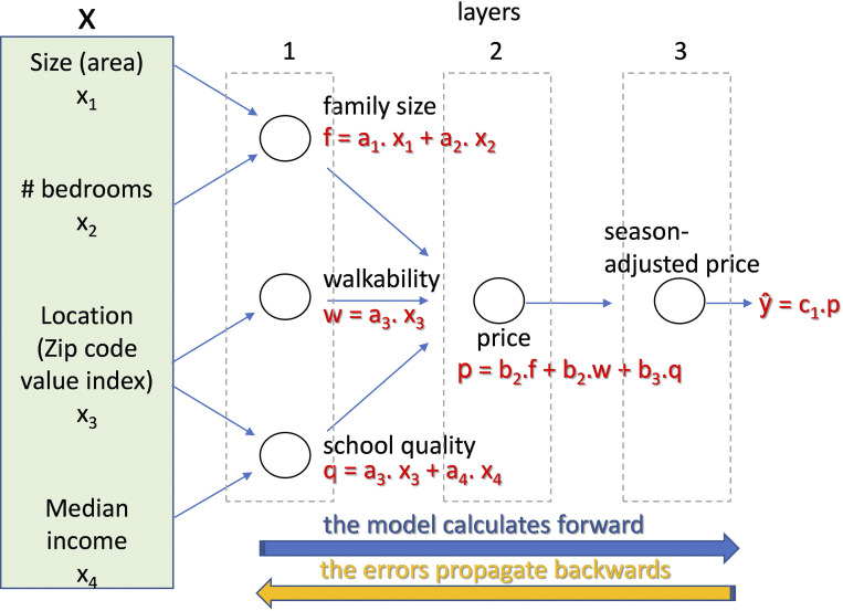
The Realtor’s network estimates the price of a home based on its features. In this simplified version, the features are four, represented by the variables xi (i = 1–4), which can also be jointly represented by a vector [X]. In the first layer of nodes or “neurons,” the variables xi are combined with (adjustable) parameters, a.k.a. weights aj to produce a set of intermediate variables (f, q, w). A second layer, containing a single neuron in the example, combines the variables again, using weights bk, to produce an estimate of price, p. p is further modified in a third layer, by another adjustable weight, c1, to yield the final estimate ŷ. The estimate and its error (loss) depend on every weight via functional compounding described in the text (Eq. 3). This example and figure are adaptations of elements of the CNN course by A. Ng (Ng, 2021).
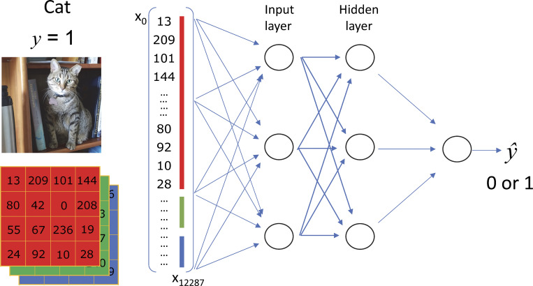
The neural networks input. A color image consists of three 2-D arrays of pixel intensities, usually in colors red, green, and blue (RGB). These values are “flattened” as shown, to a vertical array or column vector (of n[0] elements, 12,288 in the example, numbered 0–12,287 or 1–12,288, depending on conventions of the programming language), which is delivered as “input” to the first or input layer of the network (3 in the example). Every unit or neuron in this layer will combine the n[0] input values linearly, with n[0] coefficients, by the “dot product” operation, Eq. 5. The operation of all neurons in the layer produces a new vector Z[1] (Eq. 7 and Fig. 3 A). At variance with the Realtors’ example, this network is “fully connected,” or “dense.” Z is not the final output of the layer, please read on. Modified from examples and ideas in Ng (2021).
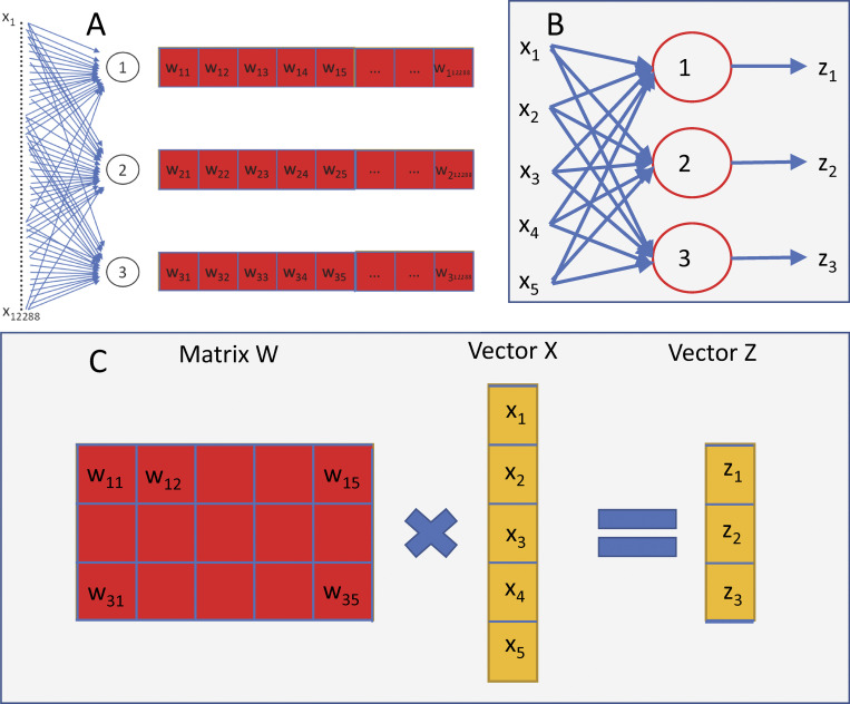
Operations of dense networks. (A) Every neuron in the first layer combines the 12,288 elements of the input image using 12,288 coefficients wij in a dot product. (B) Every neuron (3 are represented) will thus produce one component of a column vector Z. (C) The three, or generally n[1] neurons of layer 1 constitute a matrix W of n[1] rows and n[0] columns (5 and 3 in the drawing; 12,288 and 3 in the example of panel A). The operation of all neurons in the layer, graphically represented in B, is the (pre) multiplication of the vector X by the matrix W. The product, vector Z, has a number of elements (3) equal to that of rows in W. Note also that, unlike the previous examples and Eqs. 5, 6, and 7 in the text, in this figure the array indexes start at 1, a standard convention in linear algebra.
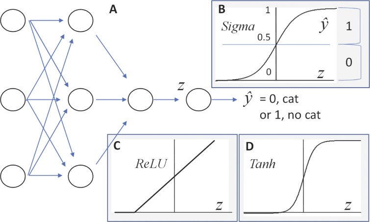
Classification. (A and B) The next-to-last layer accumulates all outputs of the previous one onto a variable z which is then processed non-linearly, via functions such as σ(z) (B). If the functional value is <0.5, the output of the network, estimate ŷ, is conventionally set to 0 (not-a-cat) in this binary case. Of course, values >0.5 lead to the alternative estimate (1). (C) ReLU is an unbounded nonlinear function that can be used to follow matrix multiplication in the hidden layers of the network. (D) Tanh, the hyperbolic tangent, is another example of functions that can be used for the final stage.
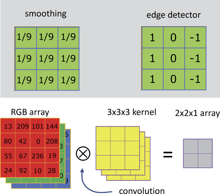
Convolutions. Top: Examples of convolution kernels or filters. The one at left performs the simplest 2-D smoothing operation, the one at right will mark vertical edges. Bottom, in a multichannel case (third dimension >1) the kernel (yellow) must have the same number of channels than the input array (3 in the example). A kernel of 3 × 3 × 3 can only be placed at four locations on this 4 × 4 × 3 input image (i.e., those centered at pixels with values 42, 0, 67, and 236 in the red array). Hence the output will be the small 2 × 2 × 1 array in gray, a case of “downsampling.” The shrinkage can be avoided by the “padding” operation, whereby rows and columns are added to the input image.
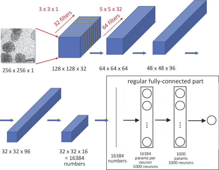
A representative convolutional neural network (modified from diagrams used in online courses by
https://Coursera.org ). Of note: The input images in successive layers are processed by multiple filters per layer; this gives rise to a third dimension in the intermediate images (which constitute tensors—volumes in blue). The dimensions of filters are listed in red font, those of the image (a.k.a. feature) tensors in black. Note consistent reduction in dimensions 1 and 2, achieved by “striding,” i.e., skipping pixels during convolutions, and increase in dimension 3 (in which components are called channels). Only the last three layers are “dense.” The transition requires flattening of the last information tensor into a vertical vector, of 16,384 elements in the example (flattening is introduced with Fig. 2). The example also shows how convolutional layers only combine nearby pixels, while dense layers may combine remotely located features in the intermediate images, at the cost of a much greater number of parameters.
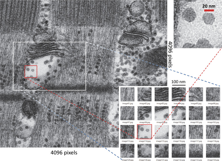
Example approach to categorical classification. An ultrathin section of a human leg muscle (biopsy provided by S. Riazi of the Malignant Hyperthermia Investigation Unit, Toronto General Hospital, Toronto, Canada) was stained for glycogen and EM-imaged by M. Samsó (Virginia Commonwealth University). The image at left comprises a portion of the interior of a cell or myofiber. It shows parts of two myofibrils (recognizable by lengthwise striations), as well as sarcoplasmic reticulum and other organelles in the space between myofibrils, with glycogen granules revealed by the staining. EM images are split into sub-images of 256 × 256 pixels and 102.4 nm sides. The set at bottom right results from splitting the area of the original within the white frame. As illustrated, sub-images are sufficiently small, in most cases, to be fully within a region of interest within the myofiber, and seldom contain more than nine glycogen granules, thus simplifying the task of the granule counting module. Reprinted from Ríos et al. (2024), Data S1.
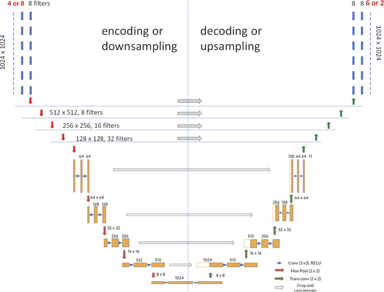
Semantic segmenters. Two structures were developed by Ríos et al. (2024) for their segmenters, starting from the conventional U-Net (section colored orange, simplified from Ronneberger et al. [2015], Preprint). The models consist of two arms (“encoding” and “decoding”) each comprising eight conv blocks (horizontal sequences of three layers, represented by rectangles). In the encoding arm, the first two layers of a block are simple convolutions, with numbers of filters that double at every block. The third is a Max Pooling operation, see red arrows, which reduces the spatial dimensions by a factor of 2. The decoding arm symmetrically recovers image size, with the expansion of dimensions produced by the “transpose convolution” operation, see blue arrows, illustrated in Fig. 9. At every level, the decoding block also incorporates images (channels) from the corresponding level of the encoding arm (represented by open rectangles), which are simply stacked to the channels generated by decoding (the “concatenate” operation, grey arrows). Locations and Granules segmenters differ only in their first and last layers (numbers in red). See also Ríos et al. (2024) Data S2 for an alternative, layer-by-layer representation.
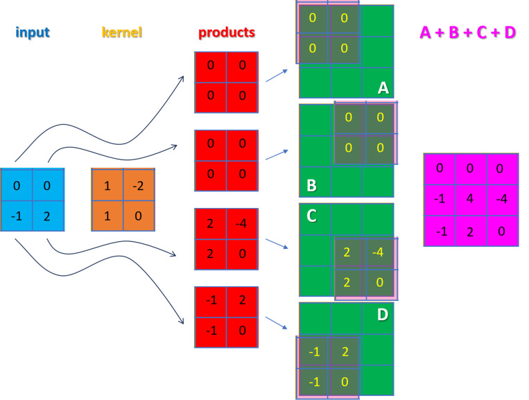
The Transposed Convolution: an operation that achieves expansion of spatial images. In the example, a 2 × 2 input (blue) is expanded to a 3 × 3 output (purple) using a kernel or filter (orange). The kernel elements are multiplied by each of the input elements to yield intermediate product arrays (red). For example, the top array in red is the result of multiplying the kernel by 0. These arrays are placed at the four corners of the 3 × 3 buffer (green) to generate terms (A–D) that are added to build the final output. For example, the central element in the output array is calculated as the sum, 0 + 0 + (2) + (2), of the corresponding elements in the buffer arrays.
References
-
- Abadi, M., Barham P., Chen J., Chen Z., Davis A., Dean J., Devin M., Ghemawat S., Irving G., Isard M., et al. 2016. TensorFlow: A system for large-scale machine learning. arXiv. 10.48550/arXiv.1605.08695 (Preprint posted May 30, 2016). - DOI
-
- Baylor, S. 2021. Computational Cell Physiology. Second edition. Self-published, Chicago, IL, USA. p. 518.
-
- Csurka, G., Volpi R., and Chidlovskii B.. 2023. Semantic image segmentation: Two decades of research. arXiv. 10.48550/arXiv.2302.06378 (Preprint posted February 13, 2023). - DOI
-
- Ham, D., Park H., Hwang S., and Kim K.. 2021. Neuromorphic electronics based on copying and pasting the brain. Nat. Electron. 4:635–644. 10.1038/s41928-021-00646-1 - DOI
MeSH terms
Grants and funding
LinkOut - more resources
Full Text Sources