Review
. 2024 Oct 17;128(41):9976-10042.
doi: 10.1021/acs.jpcb.4c04100. Epub 2024 Sep 20.

CHARMM at 45: Enhancements in Accessibility, Functionality, and Speed

Wonmuk Hwang  1   2   3   4 Steven L Austin  5 Arnaud Blondel  6 Eric D Boittier  7 Stefan Boresch  8 Matthias Buck  9 Joshua Buckner  10 Amedeo Caflisch  11 Hao-Ting Chang  12 Xi Cheng  13 Yeol Kyo Choi  14 Jhih-Wei Chu  15 Michael F Crowley  16 Qiang Cui  17   18   19 Ana Damjanovic  20   21   22 Yuqing Deng  23 Mike Devereux  7 Xinqiang Ding  24 Michael F Feig  25 Jiali Gao  26   27   28 David R Glowacki  29 James E Gonzales 2nd  1   22 Mehdi Bagerhi Hamaneh  9 Edward D Harder  30 Ryan L Hayes  31   32 Jing Huang  33 Yandong Huang  34 Phillip S Hudson  5   35 Wonpil Im  14 Shahidul M Islam  36 Wei Jiang  37 Michael R Jones  22 Silvan Käser  7 Fiona L Kearns  5 Nathan R Kern  14 Jeffery B Klauda  38 Themis Lazaridis  39 Jinhyuk Lee  40   41 Justin A Lemkul  42 Xiaorong Liu  10 Yun Luo  43 Alexander D MacKerell Jr  44 Dan T Major  45 Markus Meuwly  7   46 Kwangho Nam  47 Lennart Nilsson  48 Victor Ovchinnikov  49 Emanuele Paci  50 Soohyung Park  14 Richard W Pastor  22 Amanda R Pittman  5 Carol Beth Post  51 Samarjeet Prasad  22 Jingzhi Pu  52 Yifei Qi  53 Thenmalarchelvi Rathinavelan  54 Daniel R Roe  22 Benoit Roux  55 Christopher N Rowley  56 Jana Shen  44 Andrew C Simmonett  22 Alexander J Sodt  57 Kai Töpfer  7 Meenu Upadhyay  7 Arjan van der Vaart  5 Luis Itza Vazquez-Salazar  7 Richard M Venable  22 Luke C Warrensford  5 H Lee Woodcock  5 Yujin Wu  10 Charles L Brooks 3rd  10 Bernard R Brooks  22 Martin Karplus  49   58
Affiliations
Review

CHARMM at 45: Enhancements in Accessibility, Functionality, and Speed

Wonmuk Hwang et al. J Phys Chem B. .

Abstract

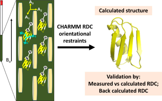
Since its inception nearly a half century ago, CHARMM has been playing a central role in computational biochemistry and biophysics. Commensurate with the developments in experimental research and advances in computer hardware, the range of methods and applicability of CHARMM have also grown. This review summarizes major developments that occurred after 2009 when the last review of CHARMM was published. They include the following: new faster simulation engines, accessible user interfaces for convenient workflows, and a vast array of simulation and analysis methods that encompass quantum mechanical, atomistic, and coarse-grained levels, as well as extensive coverage of force fields. In addition to providing the current snapshot of the CHARMM development, this review may serve as a starting point for exploring relevant theories and computational methods for tackling contemporary and emerging problems in biomolecular systems. CHARMM is freely available for academic and nonprofit research at https://academiccharmm.org/program.


Conflict of interest statement

The authors declare the following competing financial interest(s): Alexander D. MacKerell, Jr. is Co-founder and CSO of SilcsBio LLC.
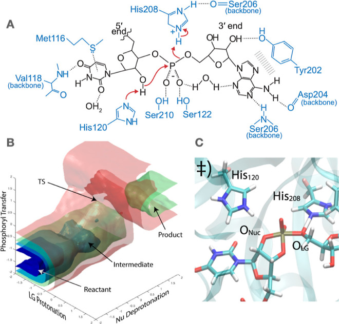
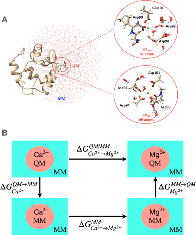
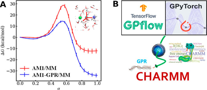
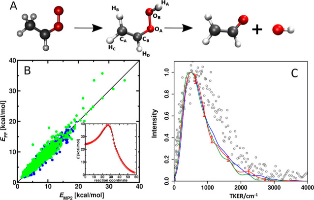
Figures

Figure 1
Figure 1
Main concepts of EnzyDock applied to the mechanism in the Diels–Alderase enzyme, LepI., (A) Similar (mapped) atoms are marked in green. (B) EnzyDock docking with the transition state as a template (“seed”) for docking the remaining states.
Figure 2
Figure 2
Thermodynamic cycle. Inset: general cycle design; horizontal arrows: measured affinities in kcal/mol;, vertical arrows: computations for tetramer (left) and the two types of dimers (right). Graphical panels: local molecular surface at the interfaces with the mutated residues displayed as spheres for WT (S59: red, H62: blue), S59A/H62L (A59: red, L62: yellow), and S59A/H62F (A59: red F62: green). For WT, a 0.41-kcal/mol entropic term is added to account for higher symmetry. Computed (C:), measured (M:) differences, and discrepancies (D:) are given. Global discrepancy (ΔΔΔG) for the 3 cycles provides a self-consistency check. Average standard deviation (StdDevcalc) and error (⟨error⟩calc) were computed using autocorrelation functions considering λ windows as independent. The average error ⟨error⟩obs and the maximum observed error Maxerror-obs that compare experimental results with calculations are also reported.
Figure 3
Figure 3
Integration along the thermodynamic cycles in Figure 2. Cumulative error estimates are also shown for the tetramer, each of the dimers, the sum of the dimers, and the global cycle for (A) WT to S59A/H62L, (B) WT to S59A/H62F, and (C) S59A/H62L to S59A/H62F for which only one dimer is involved since residue 59 remains as Ala. (D) Integrand for the transformation of the tetramer from WT to S59A/H62L shown in black as an example. The average for each λ window is marked by a stepwise white line. Linear regression along the whole trace is shown as a light gray line to appraise the linearity of the integrand with respect to λ. Dashed lines mark ±100 kcal/mol. (E) Integrand for isolated hybrid residues (acetylated and aminated) in a vacuum to evaluate the intrinsic energy contributions due to the FF energy difference of the original residues.
Figure 4
Figure 4
Illustration of the SM on the 2D Mueller potential. An MEP (dotted white curve) and a finite temperature string (solid white curve) connect the reactant (R; q = 0) and product states (P; q = 1) enclosed within red ellipses. Black contours represent isocommittor surfaces obtained from a 2nd order finite difference solution of the backward Kolmogorov equation for overdamped Langevin dynamics. White straight lines are planar approximations to the isocommittor surfaces, which also partition the configurational space into a Voronoi tessellation with nodes (red bullets). Gray dots are simulation coordinates from overdamped Langevin dynamics restrained to reaction coordinate planes and collectively define a transition tube.
Figure 5
Figure 5
Illustration of ABPO. (A) Energy landscape in the CV space at the initial stage of path optimization. Multiple trajectories are launched from the two end-state energy wells (blue) and sample freely along an arbitrary initial path (red line) enhanced by Vb and within a tube centered on the path (white transparent rectangle) by a tube potential. (B) Trajectory visits to hyperplanes (small gray rectangles) perpendicular to the path tangent are counted. After sufficient sampling, the mean position in each hyperplane from counts over all replicate trajectories (blue X’s) is determined, and the path and tube center are updated to these new values in CV space. The process is repeated to move the path incrementally (dashed arrows) until convergence to the optimal one (white curve).
Figure 6
Figure 6
In BXD, the range of values assumed by the CV ρ is partitioned in boxes separated by reflective boundaries.
Figure 7
Figure 7
End-to-end distance (ξ) over time and the PMF of deca-alanine obtained using eABF.
Figure 8
Figure 8
(A) 9-charge symmetry-constrained MDCM for CCl4. Red and blue points respectively correspond to negative and positive charge positions. A charge at the C-atom nuclear position is hidden. (B) DFT reference ESP (kcal/[mol·e]) mapped onto the 0.001 au molecular isodensity surface (left); fitted multipolar model truncated at quadrupole (middle); 9-charge MDCM model (right, root-mean-square error (RMSE) of 0.29 kcal/mol over the grid used for fitting).
Figure 9
Figure 9
Illustration of pore shapes in IMM1. (A) Constant radius. (B) Radius depending on the z-coordinate.
Figure 10
Figure 10
Illustration of the PRIMO CG model. (A) PRIMO interaction sites (red spheres) for asparagine as an example. (B) Hybrid all-atom/CG model of a protein with coupling between a PRIMO region and an atomistic region.
Figure 11
Figure 11
Helical reaction coordinates., The tilt angle τ is relative to the z-axis; the rotation angle ρ is measured for a designated atom about the helical axis; the bend angle θ is between two helical axes; the minimum distance D and crossing angle Ω are between two neighboring helices. Corresponding restraint energy functions are handled by the CONSHELIX module in CHARMM. For a hairpin, tilt, rotation, and distance restraint potentials are also available.
Figure 12
Figure 12
Structural changes of the fd-coat membrane protein through MD simulations with the SSNMR restraint potential. (A) The fd-coat system. IP (blue): In-plane helix; TM (red): Transmembrane helix. (B) Distribution of chemical shift (x-axis) and dipolar coupling (y-axis) calculated for the initial state structure. (C) Structure and calculated distribution in an intermediate stage of the simulation. Note changes in the distributions and conformations. (D) The final stage of the simulation. IP is at the lipid–water interface, while TM is positioned within the membrane.
Figure 13
Figure 13
From RDC (DPQ) measurement to structure calculation using CHARMM illustrated by using the N–H internuclear vector of protein G (PDB 1P7E). The protein solution in the NMR tube is indicted in green. Oval-shaped slabs indicate the alignment media. B0 is the applied static magnetic field, and Ai and Mi (i = 1, 2, 3) represent the 3 principal axes for the alignment tensor and the inertia tensor of the molecule, respectively.
Figure 14
Figure 14
Performance of QM/MM methods. (A) Wall time in hours per 1-ns MD simulation for insulin receptor kinase versus the number of CPU cores, for the MM-only, SQUANTM, MNDO97 BOMD, and MNDO97 with DXL-BOMD methods. (B) Energy conservation in different SCF accelerator implementations for adenylate kinase, showing less than 1 kcal/mol deviation of the total energy during 100-ps NVE MD simulations. Simulation systems consist of (A) 76 QM atoms and 28,823 MM atoms and (B) 92 QM atoms and 47,201 MM atoms. In both cases, the QM region is treated with the AM1/d-PhoT SE QM model for the MNDO97 module and with the AM1 model for the SQUANTM module.
Figure 15
Figure 15
PMF for the SN2 reaction between CH3Cl and Cl in water. Results from MTS simulations with varying number of MD steps N, for evaluating the AI-QM/MM correction term. The MTS AI-QM/MM simulations were carried out using the AM1 and HF/3-21G methods for the low- and high-level QM theories, respectively. “AM1 only” results are from the AM1 SE-QM/MM simulations. The inset compares the impact of low-level QM theory on the PMF, while the high-level theory remains at the HF/3-21G level.
Figure 16
Figure 16
Hydride transfer reaction in dihydrofolate reductase. (A) Reaction mechanism. (B) Classic (solid line) and quantum (dashed lines) PMFs for hydride and deuteride transfer. (C) Active site for the hydride transfer from NADPH to H2 folate. The transferring hydride is described using PI with 32 beads.
Figure 17
Figure 17
DFTB3/MM free energy simulations for the catalysis in Usb1. (A) The putative catalytic mechanism of Usb1. (B) The 3D free energy surface from DFTB3/MM multiwalker metadynamics simulations. The three CVs describe proton transfers associated with the catalytic acid/base and the phosphoryl transfer (red arrows in panel A). (C) The transition state structure from the DFTB3/MM free energy simulations features the transfer of a single proton between H208 and the leaving group. This was subsequently confirmed with proton inventory experiments. Panels A and C were adapted from ref (690), which was published by the Oxford University Press.
Figure 18
Figure 18
DFTB3/MM FEP simulations for the Ca2+/Mg2+ binding selectivity in the Ca2+ binding protein, carp parvalbumin (CP), and its mutant (D51A/E101D/F102W). (A) The DFTB3/MM-GSBP setup that illustrates the QM regions for the WT and mutant CP simulations. (B) Thermodynamic cycle used to probe the free energy change for the Ca2+/Mg2+ conversion in a given environment. In simulations, the horizontal transitions occur at the MM level, and in the vertical transitions, a metal binding site is converted between MM and QM treatments using the PERT module in CHARMM. Reproduced from ref (691). Copyright [2024] American Chemical Society.
Figure 19
Figure 19
(A) PMFs of the Menshutkin reaction (NH3 + CH3Cl → NH3CH3+ + Cl) simulated at the AM1/MM and AM1-GPR/MM levels. (B) The scheme of combining GPR Python libraries and CHARMM through pyCHARMM.
Figure 20
Figure 20
(A) OH-elimination following vibrational excitation of syn-CH3CHOO. (B) Performance of MS-ARMD. The RMSEs between reference ab initio energies and the fitted FF for reactant (blue) and product (green) are 1.1 and 1.2 kcal/mol, respectively. Inset: MEP calculated with MS-ARMD (red circles) compared with reference calculations (black line). (C) Distribution of the total kinetic energy release from several thousand trajectories following CH-excitation with ∼2 quanta using the MS-ARMD PES with OO scission energies of 22, 25, and 27 kcal/mol (blue, red, green). Open symbols are experimental results. Panels A and B reproduced from ref (382). Copyright [2021] American Chemical Society.
Figure 21
Figure 21
Illustration of an indirect cycle to compute a free energy difference at the QM/MM level of theory.
Figure 22
Figure 22
MSD vs t for 1-μs NVT and NPT simulations of 1340 TIP3P waters. The plots are offset by intervals of 0.25 × 10⁶ Å2 on the y-axis to better distinguish them. From top to bottom, violet: NPT with Cartesian unwrapping; green: NPT with toroidal view preserving scheme; orange: NVT with Cartesian unwrapping; blue: NPT with unwrapping in fractional space and using average unit cell vectors (CHARMM XFLUC); black: NPT with unwrapping in fractional space (CHARMM method). Trajectories were run with OpenMM and analyzed with CPPTRAJ version 6.19.3.
Figure 23
Figure 23
Probabilities of wrap counts for water molecules from a 1-μs NPT MD simulation of TIP3P water and for a bilayer containing 288 DPPC molecules from 5 replicate 400-ns MD simulations. The inset omits the large peak for DPPC with zero wraps; the mean number of lipid wrap counts is 111.5.
Figure 24
Figure 24
(A) Comparison of pressure profiles from a 100-ns CHARMM simulation of palmitoylsphingomyelin bilayer with complete sampling (Direct) or via the 10% resampling (Resamp) of 100-ps intervals spaced 1-ns apart, using restart files from the fully sampled simulation. The values of the first moment and their standard errors are 0.190 ± 0.009 and 0.192 ± 0.004, respectively. (B) Pressure profiles of a bilayer composed of 72 1,2-dipalmitoyl-sn-glycero-3-phosphocholine at 1 atm and 323 K. Data from resampling were obtained by the binning method with 100 bins from the previous CHARMM simulations (black), where 100-ps resampling was done for every 1 ns. Post analysis using single-step dynamics was tested using 500-ns OpenMM NPT trajectories of the same bilayer, where the pressure profiles were calculated for each frame by both the binning (blue) and Fourier series (red) methods. The numbers of bins and Fourier coefficients were set to 80 and N = 20 (Eq. 73), respectively. Standard errors from five 100-ns blocks are shown in cyan and pink areas, respectively, which are smaller than the line thickness except near dips. (C) Pressure profiles for a 1,2-dinervonoyl-sn-glycero-3-phosphocholine bilayer with a model peptide of 9 monomeric units of gramicidin A in the upper leaflet at a peptide area fraction ϕ ∼ 0.40 before (red) and after P21 equilibration (black). The P21 PBC in CHARMM allows lipid translocation between bilayer leaflets, which reduces area stress and alters the lateral pressure profile (see Section 12.4). The bilayer midplane was set to z = 0. Pressure profiles from the last 300-ns trajectories of 5 replicas from OpenMM were averaged for each asymmetric bilayer, whose standard errors are shown as pink and gray areas (typically smaller than the line thickness). Pressure profiles were calculated by single-step dynamics for each frame of trajectories with 200 bins along the z-direction. Panel A reproduced from ref (804). Copyright [2014] Cell Press. Panel C reproduced from ref (44). Copyright [2023] Wiley.

References

    1. McCammon J. A.; Gelin B. R.; Karplus M. Dynamics of folded proteins. Nature 1977, 267, 585–90. 10.1038/267585a0. - DOI - PubMed
    1. Macuglia D.; Roux B.; Ciccotti G. The emergence of protein dynamics simulations: how computational statistical mechanics met biochemistry. Euro. Phys. J. H 2022, 47, 13.10.1140/epjh/s13129-022-00043-y. - DOI
    1. Brooks B. R.; Brooks C. L. III; MacKerell A. D. Jr.; Nilsson L.; Petrella R. J.; Roux B.; Won Y.; Archontis G.; Bartels C.; Boresch S.; et al. CHARMM: the biomolecular simulation program. J. Comput. Chem. 2009, 30, 1545–1614. 10.1002/jcc.21287. - DOI - PMC - PubMed
    1. Brooks B. R.; Bruccoleri R. E.; Olafson B. D.; States D. J.; Swaminathan S.; Karplus M. CHARMM - a program for macromolecular energy, minimization, and dynamics calculations. J. Comput. Chem. 1983, 4, 187–217. 10.1002/jcc.540040211. - DOI
    1. Harris J. A.; Liu R.; de Oliveira V. M.; Vázquez-Montelongo E. A.; Henderson J. A.; Shen J. GPU-accelerated all-atom particle-mesh Ewald continuous constant pH molecular dynamics in Amber. J. Chem. Theory Comp. 2022, 18, 7510–7527. 10.1021/acs.jctc.2c00586. - DOI - PMC - PubMed