Abnormal hyperactivity of specific striatal ensembles encodes distinct dyskinetic behaviors revealed by high-resolution clustering

Abstract

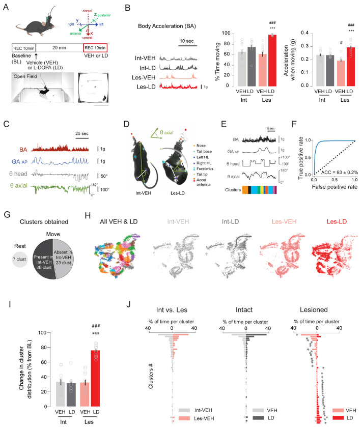
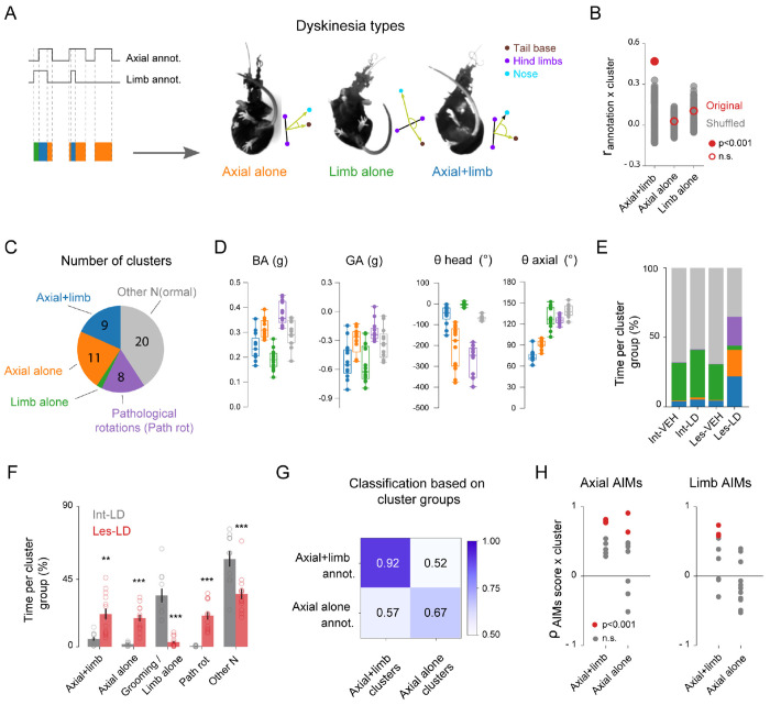
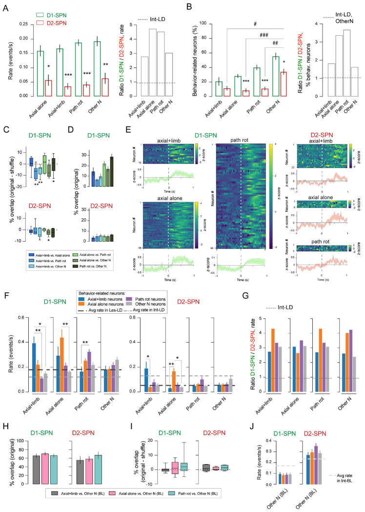
L-DOPA-induced dyskinesia (LID) is a debilitating complication of dopamine replacement therapy in Parkinson's disease and the most common hyperkinetic disorder of basal ganglia origin. Abnormal activity of striatal D1 and D2 spiny projection neurons (SPNs) is critical for LID, yet the link between SPN activity patterns and specific dyskinetic movements remains unknown. To explore this, we developed a novel method for clustering movements based on high-resolution motion sensors and video recordings. In a mouse model of LID, this method identified two main dyskinesia types and pathological rotations, all absent during normal behavior. Using single-cell resolution imaging, we found that specific sets of both D1 and D2-SPNs were abnormally active during these pathological movements. Under baseline conditions, the same SPN sets were active during behaviors sharing physical features with LID movements. These findings indicate that ensembles of behavior-encoding D1- and D2-SPNs form new combinations of hyperactive neurons mediating specific dyskinetic movements.

Keywords: L-DOPA-induced dyskinesia; accelerometer; calcium imaging; freely-moving mouse behavior; inertial measurement units; striatal activity; unsupervised behavioral clustering.

Figure 1.. Behavioral changes in dyskinetic mice revealed by unsupervised behavioral clustering

(A) Illustration of the microendoscope and the wireless inertial measurement unit (IMU) placed on top of the mouse head. On the right is shown the orientation of the 6 axes of the IMU: three axes for the acceleration (x = dorso-ventral; y = posterior-anterior; z = right-left) and three axes for the gyroscope which measures the rotational velocity around these axes, represented by the rotating arrows. Below is the timeline of the experimental design (STAR Methods) and on the bottom, the view of the open field arena from the side- and bottom-placed cameras (scale bar, 20 cm). (B) Example traces of the body acceleration (BA) in the four conditions. Bar plot on the right shows the mean of the time moving as a percentage of the total time of the session ± SEM (n = 11-13 mice). Ordinary 1-way ANOVA, F_{(3, 42)} = 18.27, p < 0.001. Post hoc Bonferroni’s multiple comparisons test shows ***p < 0.001 Les-LD vs. Les-VEH; ^###p < 0.001 Les-LD vs. Int-LD. Right: Body acceleration (g) while moving ± SEM (n = 11-13 mice). Ordinary 1-way ANOVA, F(_{3, 42}) = 17.56, p < 0.001. Post hoc Bonferroni’s multiple comparisons test shows ***p < 0.001 Les-LD vs. Les-VEH; ^###p < 0.001 Les-LD vs. Int- LD; ^#p < 0.05 Les-VEH vs. Int-VEH. (C) Example traces of the four features used for the clustering: BA, GA_AP (gravitational acceleration along the antero-posterior axis), θ head (head angle, proxy of rotations) and θ axial (axial bending angle, proxy of axial AIMs; see STAR Methods). (D) Video frames showing two mice (left from Int-VEH; right Les-LD) taken with the bottom camera. Shown are the 9 tracking points labeled using DeepLabCut software. The axial bending angle, θ axial, was calculated based on the hindlimbs (HL), the tail base and nose, as in (see STAR Methods and Movie S1). Note that the Int-VEH mouse has a flat angle (~180 deg) compared to the Les-LD mouse whose θ axial is ~40 deg. (E) Behavioral clustering using BA, GA_AP, θ head and θ axial. Top: BA, GA_AP, θ head and θ axial time series. Bottom: corresponding behavioral clusters obtained by affinity propagation on similarity of discretized time series (STAR Methods). (F) Resulting clusters are well separated as indicated by a ROC analysis using a single threshold on the Earth Mover Distances (EMD). True positive are two segments belonging to the same cluster; false positive are two clusters belonging to different clusters. Original accuracy (ACC) was compared to accuracy for shuffled clusters: paired t-test, t(24) = 166.3, p < 0.001 (n = 25 mice). (G) Clustering resulted in a total of 56 clusters separated in two major groups: clusters corresponding to rest behavior (7 clusters) and to behavior when the animal is moving (move, 49 clusters). Move clusters were further subdivided into a group of clusters present in Int-VEH (26 clusters) and one absent in Int-VEH (23 clusters). (H) Two-dimensional t-SNE representation of the cluster segments. Each dot represents a behavioral segment. On the left, space representation of the VEH and LD sessions of the library (‘All VEH & LD’), each color being a different cluster. On the right, behavioral representation of the four conditions Int/VEH or LD and Les/VEH or LD. Note a very similar space representation of the segments obtained in Int-VEH, Int-LD and Les-VEH, in contrast with the ones from Les-LD. (I) Change in the cluster distributions compared to baseline (BL). Bar plot represents the percentage of change ± SEM (n = 10-13 mice). Ordinary 1-way ANOVA, F_{(3, 42)} = 43.82, p < 0.001. Post hoc Bonferroni’s multiple comparisons test shows ***p < 0.001 Les-LD vs. Les VEH; ###p < 0.001 Les-LD vs. Int-LD. (J) Left: percentage of time spent per cluster between Int-VEH and Les-VEH (Mann-Whitney U test for the 26 clusters present in Int-VEH; all p > 0.05 after Benjamini–Yekutieli post-hoc correction; n = 19 Int mice, n = 20 Les mice). Middle: percentage of time spent per cluster in Int-VEH versus Int-LD (Wilcoxon signed-rank test for all moving clusters; all p > 0.05 after Benjamini–Yekutieli post-hoc correction, n = 19 mice). Right: percentage of time spent per cluster in Les-VEH and Les-LD (Wilcoxon signed-rank test for all moving clusters; *p < 0.05 for 39 out of 49 clusters after Benjamini–Yekutieli post-hoc correction, n = 20 mice).

Figure 2.. Behavioral clustering captures specific dyskinesias and other pathological behaviors

(A) Schematic representation of the frame-by-frame annotations of axial and limb dyskinesias. Three dyskinesia types were considered for the further analyses: axial alone (orange), limb alone (green) and axial+limb simultaneously (blue, see also Movie S1). (B) Example cluster for one mouse that significantly correlated with the axial+limb annotation but not with axial alone or limb alone. Bootstrap analysis of r_{annotation x cluster} to shuffled annotations (red closed circle: p < 0.001, red open circles: not significant, see STAR Methods for details). (C) Left: summary of the behavioral cluster groups obtained after correlating the behavior cluster to the dyskinesia annotations in all n = 13 mice (see STAR Methods for details). Twenty-one clusters were significantly correlated with the dyskinesia annotations: 9 were correlated with axial+limb; 11 to axial alone and 1 was correlated with limb alone. Twenty-eight clusters were not correlated with any dyskinesia and were denoted as other N for ‘normal’ (n = 20 clusters) if the clusters were present in Int-VEH mice, and pathological rotations (path rot, n = 8) if the clusters were absent in Int-VEH. (D) Feature characteristics of the cluster groups. Box and whiskers diagrams show the values of each of the 4 features (BA, GA, θ head and θ axial) corresponding to the 5 cluster groups. Values are means ± SEM (n = 13 mice). Repeated measures 1-way ANOVA, for BA, F_{(2.666, 31.99)} = 103.5, p < 0.001; for GA, F_{(1.504, 18.05)} = 21.55, p < 0.001; for θ head, F_{(1.259, 15.11)} = 80.40, p < 0.001 and for θ axial, F_{(2.025, 24.30)} = 217.4, p < 0.001. (E) Percentage of time spent per cluster group for each condition. Note that in Int-VEH, Int-LD and Les-VEH, mice spend the majority of their time (> 50%) in the other N cluster group and around 30% of the time in the limb alone cluster, which corresponds to grooming (see also Figure S2C). In Les-LD, mice show variable time spent in each of the 5 cluster groups. (F) Detailed comparison of time spent per cluster group between Int-LD (gray) and Les-LD (red). Bar plots represent the percentage of time spent per cluster group, values are the mean ± SEM (n - 10-13 mice). Two-way repeated measures ANOVA shows an effect of the cluster groups, F_(4.84) = 39.44, p < 0.001; no effect of the lesion, F_(1,21) = 0.04, p = 0.84; and an effect of the interaction, F_{(4, 84)} = 26.11, p < 0.001. Post hoc Bonferroni’s multiple comparisons test shows **p < 0.01 and ***p < 0.001 Int-LD vs. Les-LD. (G) Accuracy of a support vector classifier for predicting the type of dyskinesia (annotation) based on the axial+limb and axial alone cluster groups (see STAR Methods for details). Classification accuracies were significantly different from shuffled data. Paired t-test, axial+limb: t(10) = 61.1, p < 0.001; axial alone: t(12) = 8.8, p < 0.001. (H) Correlation between the AIM scores and the dyskinesia cluster groups axial+limb and axial alone. Each point represents a cluster. Spearman rank-order correlation, red points are clusters that are significantly correlated with the AIM scores, p < 0.001; gray points are non-significant correlations. Note that the axial AIMs are positively correlated to some of the clusters in both the axial+limb and axial alone groups. In contrast, and as expected, limb AIMs are correlated only to clusters in the axial+limb group but not in the axial alone group.

Figure 3.. SPNs average activity is oppositely modulated by L-DOPA in 6-OHDA lesioned mice

(A) Cartoon of a mouse head showing the micro-endoscope on top of the mouse head connected to a 1 mm GRIN lens placed in the dorso-lateral striatum and the wireless IMU on the back of the micro-endoscope. On the right, coronal sections of two example mouse brains at the level of the striatum. Photomicrographs were acquired from A2a-Cre transgenic intact (A2a Int, top row) and 6-OHDA lesioned (A2a Les, bottom row) mice injected intrastriatally with the AAV5-GCamP6f viral vector. GFP expression (revealed with GFP antibody in green) in the dorso-lateral striatum shows the region of the striatum transduced with AAV5-GCamP6f viral vector, which is expressed below the 1 mm lens. TH (tyrosine hydroxylase, in red) shows the dopamine terminals in the striatum (note that A2a Les has a complete dopamine depletion shown by the lack of TH immunostaining in the right striatum). Merged photograph shows colocalization of GFP and TH showing the expression of GCamP6f in an intact (top) and a lesioned striatum (bottom) (scale bar: 1 mm). (B) Field of view of the striatum (striatal F.O.V.) through the lens of a D1-Cre lesioned mouse treated with LD, corresponding to a maximum projection of 3000 frames of the video recording. Fluorescent calcium signal shows increased fluorescence in neuronal somas (example neurons depicted by the arrows) and lack of fluorescence of a blood vessel (shown by an asterisk). Right picture shows the same F.O.V. with the total number of neurons (283 neurons) detected with the CNMFe algorithm during both BL and LD sessions, shown as footprints or ROIs (regions of interest) colored in green (scales: 60 μm). (C) Event rate of D1-SPNs in Int and Les mice treated with VEH and LD. On the left, example traces of n = 3 neurons of Int (gray, top row) and n = 3 neurons of Les (red, bottom row) mice (scale bar: 200 sec). First column corresponds to traces at BL and after VEH and the second column shows traces at BL and after LD (note that BL and VEH/LD are separated by a dashed line). Bar graph represents the average of the event rates (events/s) per mouse and session when moving (move) ± SEM (n = 3-7 mice per group and 6 to 18 sessions per group). Ordinary 1-way ANOVA, F_{(3, 18)} = 15.60, p < 0.001. Post hoc Bonferroni’s multiple comparisons test shows ***p < 0.001 Les-LD vs. Les-VEH; # p < 0.05 Les-LD vs. Int-LD; ^##p < 0.005 Les-VEH vs. Int-VEH. The bar graph on the right shows the event rates when the mice are at rest. Note that the Les-LD group is not represented because Les-LD mice did not rest (see STAR Methods). Ordinary 1-way ANOVA, F_{(2, 12)} = 1.889, p = 0.1936 (see Movie S3 for D1-SPN calcium imaging aligned to the video camera recording). (D) Event rate of D2-SPNs in Int and Les mice treated with VEH and LD. On the left, example traces of n = 3 neurons of Int and Les mice as in (C). Bar graph represents the average of event rates (events/s) per mouse and session ± SEM (n = 6 mice per group and 8 to 14 sessions per group). Ordinary 1-way ANOVA, F_{(3, 20)} = 10.59, p = 0.0002. Post hoc Bonferroni’s multiple comparisons test shows ***p < 0.001 Les-LD vs. Les-VEH; #p < 0.05 Les-LD vs. Int LD. Bar plot on the right shows the event rates when mice are at rest. Ordinary 1-way ANOVA, F_{(2, 15)} = 29.11, p < 0.001. Post hoc Bonferroni’s multiple comparisons test shows ^###p < 0.001 Les-VEH vs. Int-VEH (see Movie S4 for D2-SPN calcium imaging aligned to the video camera recording). (E) Number of active (detected with CNMFe algorithm) D1-SPNs in Int and Les mice treated with VEH and LD when mice were moving. The plots show the number of active neurons ± SEM (n = 3-7 mice per group and 6 to 18 sessions per group). Ordinary 1-way ANOVA, F_{(3, 19)} = 3.561, p = 0.0338. Post hoc Bonferroni’s multiple comparisons test shows *p < 0.05 Les-LD vs. Les-VEH. (F) Number of active D2-SPNs in Int and Les mice treated with VEH and LD. The plots show the number of active neurons ± SEM (n = 6 mice per group and 8 to 14 sessions per group). Ordinary 1-way ANOVA, F_{(3, 20)} = 3.134, p = 0.0484. Post hoc Bonferroni’s multiple comparisons test shows *p < 0.05 Les-LD vs. Les-VEH. (G) Spatiotemporal cross-correlation between pairs of active SPNs of Les mice after VEH vs. LD. For D1-SPNs, two-way repeated measures ANOVA shows an effect of the distance, F_(8,54) = 195.9, p < 0.001; no effect of the treatment, F_(1,54) = 0.0088 , p = 0.9257; and an effect of the interaction, F_{(8, 54)} = 2.421, p = 0.0259. Post hoc Bonferroni’s multiple comparisons test shows **p < 0.01 at 31 μm distance between VEH and LD (squared inset from 30 to 73μm). For D2-SPNs, two-way repeated measures ANOVA shows an effect of the distance, F_(8,45) = 108.5, p < 0.001; the treatment, F_(1,45) = 8.651 , p = 0.0051; and the interaction, F_{(8, 45)} = 2.750, p = 0.0146. Post hoc Bonferroni’s multiple comparisons test shows ***p < 0.001 at 31 μm distance between VEH and LD (squared inset from 30 to 73μm). (H) Comparison of the spatiotemporal cross-correlation between pairs of active D1-SPNs vs. D2-SPNs of Les mice after LD. Two-way repeated measures ANOVA shows an effect of the distance, F_(8,88) = 193.8, p < 0.001; a smaller effect of the treatment, F_(1,11) = 4.984 , p = 0.0473; and an effect of the interaction, F_(8,88) = 4.741, p < 0.001. Post hoc Bonferroni’s multiple comparisons test shows ***p < 0.001 at 31 μm distance between D1-SPN and D2-SPN. (I) Comparison of the spatiotemporal cross-correlation between pairs of active D1-SPNs vs. D2-SPNs of Les mice after VEH. Two-way repeated measures ANOVA shows an effect of the distance, F_(8,88) = 246.5, p < 0.0001; no effect of the treatment, F_(1,11) = 0.4845 , p = 0.5008; and an effect of the interaction, F_(8,88) = 2.92, p < 0.01. Post hoc Bonferroni’s multiple comparisons test shows no significant difference at any distance between D1-SPN and D2-SPN.

Figure 4.. Specific sets of D1-SPNs and D2-SPNs are associated with the dyskinesia clusters

(A) Left: average event rate of all D1-SPNs and all D2-SPNs during each behavioral cluster group in Les-LD mice. The bar plots represent the mean ± SEM (n = 6-7 mice, 2-3 sessions per mouse) of D1-SPNs (green) and D2-SPNs (red) event rates (events/s) in axial+limb, axial alone, path rot, other N cluster groups. Two-way repeated measures ANOVA: SPN type, F_{(1, 11)} = 49.31, p < 0.001; Cluster group, F_{(2.154, 23.69)} = 3.004 , p = 0.0654; interaction, F_{(3, 33)} = 2.021, p = 0.13. Post hoc Bonferroni’s multiple comparisons test shows *p < 0.05 D1-SPN vs. D2-SPN in axial+limb cluster group; ***p < 0.001 D1-SPN vs. D2-SPN in axial alone and path rot cluster group, and **p < 0.01 D1-SPN vs. D2-SPN in other N. Right: ratio of the event rate in D1-SPN vs. D2-SPN per cluster group. Dashed line is the ratio between D1-SPN and D2-SPN average rate in Int-LD during move. (B) Left: percentage of behavior-related D1-SPNs and D2-SPNs in Les-LD mice (a neuron is defined as behavior-related if it showed a significant positive correlation between its activity and the behavior, see STAR Methods). The bar plots represent the mean ± SEM (n = 6-7 mice, 2-3 sessions per mouse) of the percentage of neurons significantly modulated in axial+limb, axial alone, path rot, and other N cluster groups. Dashed line is the ratio between D1-SPN and D2-SPN’s % of behavior-related neurons in Int-LD during other N cluster groups. Two-way repeated measures ANOVA: SPN type, F_{(1, 11)} = 61.44, p < 0.001; Cluster group, F_{(1.650, 18.15 )} = 23.20 , p < 0.001; interaction, F_{(3, 33)} = 2.253, p = 0.1005. Post hoc Bonferroni’s multiple comparisons test shows: ***p < 0.001 D1-SPN vs. D2-SPN in axial alone and path rot cluster group; *p < 0.05 D1-SPN vs. D2-SPN in other N cluster group; in D2-SPN ^#p < 0.05 axial+limb vs. other N; ^###p < 0.001 axial alone vs. other N; ^##p < 0.01 path rot vs. other N. Right: ratio of the behavior-related D1-SPN over D2-SPN per cluster group. Dashed line represents no changes in the ratio. (C) Percentage of shuffle-corrected overlap between behavior-related neuronal groups for D1-SPNs and D2-SPNs. The overlap was calculated as the number of neurons shared over the total number of neurons in the two respective behavioral cluster groups. This number varies between 0 (no shared neuron) and 100% (complete overlap). Shuffle corrected overlap is the overlap minus the shuffle overlap (see STAR Methods for details). Box and whiskers diagrams show the values for the overlap between all the different comparisons. Individual unpaired t-tests showed a significant difference (compared to 0), **p < 0.01: in axial+limb vs path rot and axial+limb vs other N; *p < 0.05: in path rot vs other N. (D) Percentage of overlap between the different behavioral clusters in the original data (i.e., without shuffle correction). The bar plots represent the mean ± SEM (n = 6-7 mice, 2-3 sessions per mouse). (E) Example heatmaps of individual D1-SPN (left) and D2-SPNs (right) aligned to the beginning of the behavioral events (at time point 0 s) for axial+limb, axial alone and path rot behavioral clusters, and the corresponding average curves of the z-scored DF/F. Unpaired t-test comparing time period (−1 to −0.1 sec) and (0.1 to 1 sec) shows significant difference in axial+limb, axial alone and path rot in D1-SPNs (*p < 0.05) and D2-SPNs (**p < 0.01). (F) Behavior-related D1-SPN and D2-SPN event rate during the different behavioral cluster groups. Each bar represents the average event rate ± SEM (n = 6-7 mice, 2-3 sessions per mouse) of the behavior-related neurons for each behavioral cluster group. Black dashed line is the average rate in Les-LD during move, and the gray dashed line is the average rate in Int-LD during move. Note that the behavior-related D1-SPNs and D2-SPNs show the highest activity during their respective behavior. Kruskal-Wallis nonparametric test was performed for each of the 4 cluster groups individually. Left: for D1-SPN, Kruskal-Wallis test showed significance for axial+limb (**p < 0.01), axial alone (**p < 0.01) and path rot (*p < 0.05) cluster groups, but not for other N. Post hoc Dunn’s multiple comparison shows: in axial+limb cluster group, **p < 0.01 ‘axial+limb neurons’ vs. ‘path rot neurons’ and *p < 0.05 vs. ‘other N neurons’; in axial alone cluster group, **p < 0.01 ‘axial alone neurons’ vs. ‘other N neurons’; and in path rot cluster group, **p < 0.01 ‘path rot neurons’ vs. ‘axial+limb neurons’. Right: for D2-SPN, Kruskal-Wallis test showed significance for axial alone cluster group (**p < 0.01), but not for axial+limb (p = 0.05, n.s.), path rot or other N. Post hoc Dunn’s multiple comparison shows: in axial+limb cluster group, *p < 0.05 ‘axial+limb neurons’ vs. ‘axial alone neurons’; in axial alone cluster group, **p < 0.01 ‘axial alone neurons’ vs. ‘axial+limb neurons’ and *p < 0.05 vs. other N cluster group. (G) Ratio of the event rate in D1-SPN vs. D2-SPN per cluster group. Dashed line is the ratio between D1-SPN and D2-SPN average rate in Int-LD during move. (H) Percentage of overlap between axial+limb, axial alone, path rot SPNs under LD and other N SPNs during BL, using the original data, i.e.,without shuffle correction (shown are the mean ± SEM; n = 6-7 mice, 2-3 sessions per mouse). (I) Percentage of overlap between the neuron groups in (H) with shuffle correction, calculated as in (C). Box and whiskers diagrams show the values for the overlap between all the different comparisons. Individual unpaired t-tests showed no significant difference (compared to 0) in any of the compared groups. (J) Behavior-related D1-SPNs and D2-SPNs event rate during other N during BL average event rate ± SEM; (n = 6-7 mice, 2-3 sessions per mouse). Dashed line is the average rate in Int-BL for D1-SPN and D2-SPN.

References

1. Espay A.J., Morgante F., Merola A., Fasano A., Marsili L., Fox S.H., Bezard E., Picconi B., Calabresi P., and Lang A.E. (2018). Levodopa-induced dyskinesia in Parkinson disease: Current and evolving concepts. Ann. Neurol. 84, 797–811. 10.1002/ana.25364. - DOI - PubMed
1. Luquin M.R., Scipioni O., Vaamonde J., Gershanik O., and Obeso J.A. (1992). Levodopa-induced dyskinesias in Parkinson’s disease: Clinical and pharmacological classification. Mov. Disord. 7, 117–124. 10.1002/mds.870070204. - DOI - PubMed
1. Cenci M.A., and Kumar A. (2024). Cells, pathways, and models in dyskinesia research. Curr. Opin. Neurobiol. 84, 102833. 10.1016/j.conb.2023.102833. - DOI - PubMed
1. Girasole A.E., Lum M.Y., Nathaniel D., Bair-Marshall C.J., Guenthner C.J., Luo L., Kreitzer A.C., and Nelson A.B. (2018). A Subpopulation of Striatal Neurons Mediates Levodopa-Induced Dyskinesia. Neuron 97, 787–795.e6. 10.1016/j.neuron.2018.01.017. - DOI - PMC - PubMed
1. Parker J.G., Marshall J.D., Ahanonu B., Wu Y.-W., Kim T.H., Grewe B.F., Zhang Y., Li J.Z., Ding J.B., Ehlers M.D., et al. (2018). Diametric neural ensemble dynamics in parkinsonian and dyskinetic states. Nature 557, 177–182. 10.1038/s41586-018-0090-6. - DOI - PMC - PubMed
Publication types
LinkOut - more resources