Track-A-Worm 2.0: A Software Suite for Quantifying Properties of C. elegans Locomotion, Bending, Sleep, and Action Potentials

Abstract

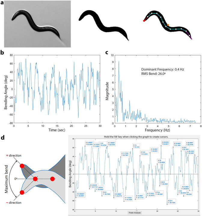
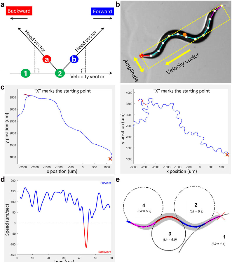
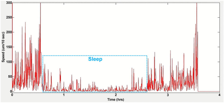
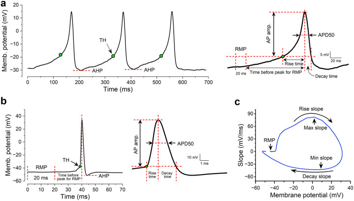
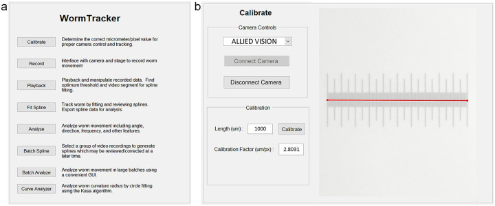
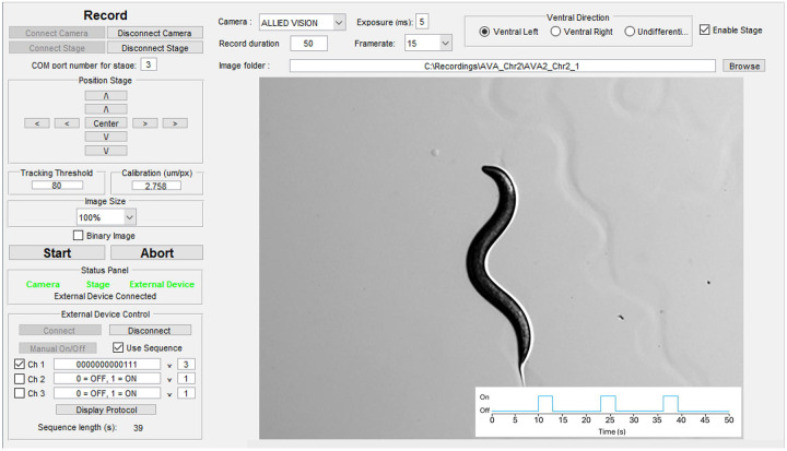
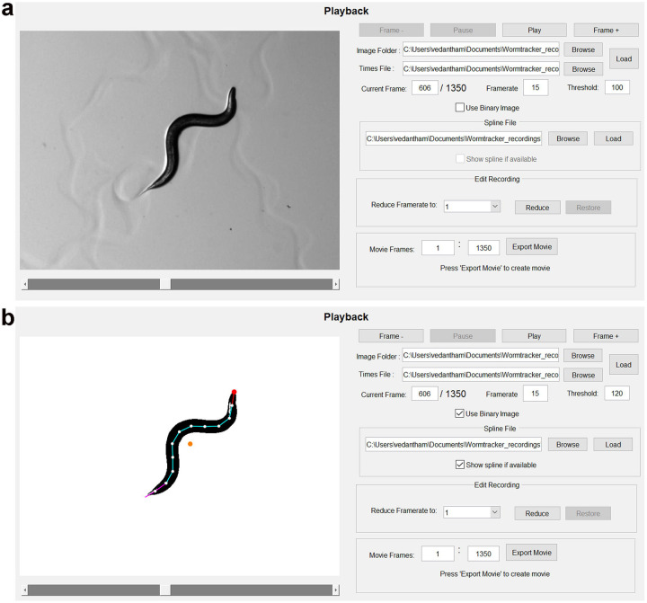
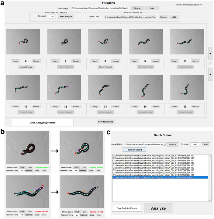
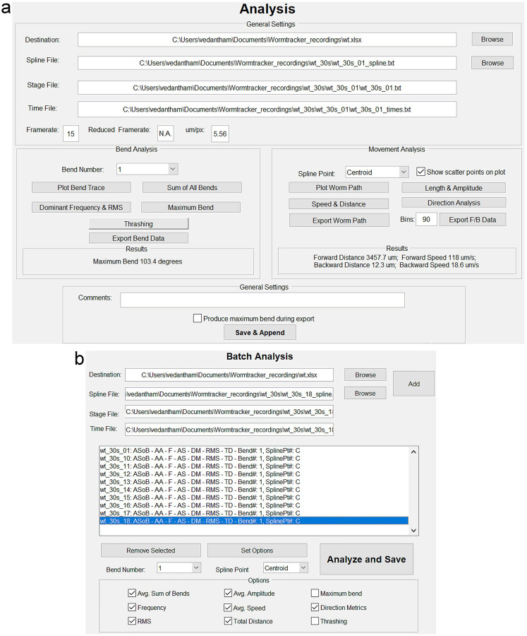
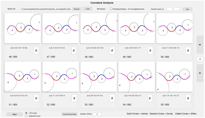
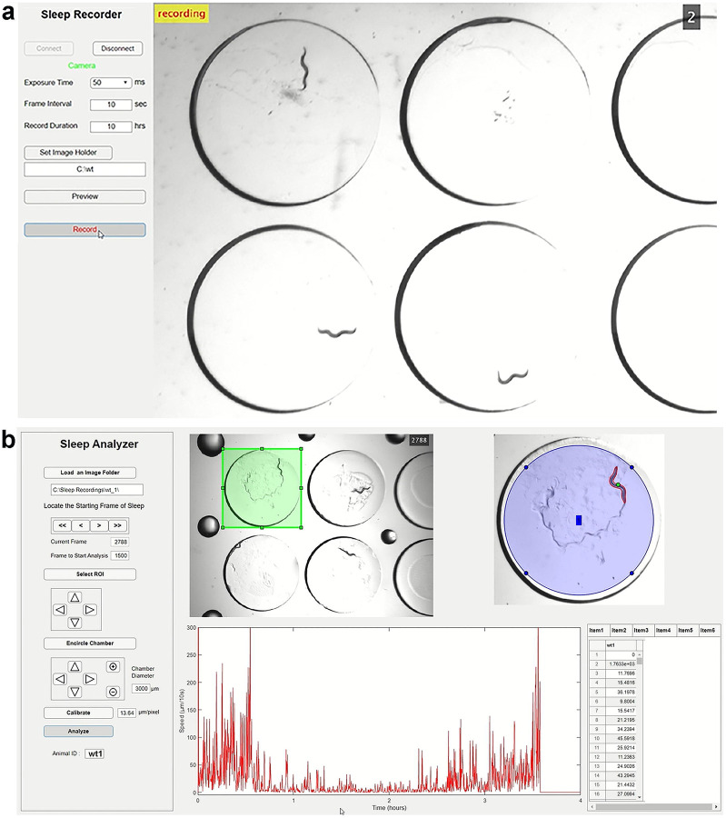
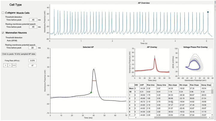
Comparative analyses of locomotor behavior and cellular electrical properties between wild-type and mutant C. elegans are crucial for exploring the gene basis of behaviors and the underlying cellular mechanisms. Although many tools have been developed by research labs and companies, their application is often hindered by implementation difficulties or lack of features specifically suited for C. elegans. Track-A-Worm 2.0 addresses these challenges with three key components: WormTracker, SleepTracker, and Action Potential (AP) Analyzer. WormTracker accurately quantifies a comprehensive set of locomotor and body bending metrics, reliably distinguish between the ventral and dorsal sides, continuously tracks the animal using a motorized stage, and seamlessly integrates external devices, such as a light source for optogenetic stimulation. SleepTracker detects and quantifies sleep-like behavior in freely moving animals. AP Analyzer assesses the resting membrane potential, afterhyperpolarization level, and various AP properties, including threshold, amplitude, mid-peak width, rise and decay times, and maximum and minimum slopes. Importantly, it addresses the challenge of AP threshold quantification posed by the absence of a pre-upstroke inflection point. Track-A-Worm 2.0 is potentially a valuable tool for many C. elegans research labs due to its powerful functionality and ease of implementation.

Figure 1.. WormTracker hardware components.

Shown are the hardware configuration of our system, including a fluorescence stereomicroscope (M165 FC, Leica) (a) with a fluorescence light source (LED3, Leica) (b), a C-mount CMOS camera (Mako G-040B, Allied Vision) (c), a motorized stage (Optiscan^™ ES111) (d) with a stage controller (ES11) (e), a joystick (CS1521DP) (f), a universal specimen holder (H473) (g), and a stage mounting bracket (H413) (h) (all from Prior Scientific), and an external device controller (myDAQ, National Instruments) (i). The WormTracker software is preconfigured to work with components c, d, and i. Components b and a 520-nm longpass cutoff filter (Y52, Hoya Corporation) are required only for optogenetic stimulation. The Petri dish is 60 mm in diameter. The yellow color in the Petri dish is due to light from the microscope base filtered through the longpass filter.

Figure 2.. Spline generation and bending property quantification.

a. Conversion of a grayscale image (left) to a binary image (middle), followed by spline fitting to the binary image (right). The spline is generated by placing 13 markers at equal intervals along the longitudinal axis of the worm’s body, with the marker at the head tip shown in red and the centroid in orange. b. Bend trace of a worm recorded over 30 seconds. c. Bending frequency spectrum of the same worm, with the dominant bending frequency and RMS (root mean square) bend angle from the Results section displayed within the graph. d. Quantification of the maximum bend. Left: Diagram illustrating the definition of the maximum bend, which is the maximum bending angle of a spline marker point in the ventral and dorsal directions relative to a straight line fitted to the two subsequent spline markers. Right: A bend trace with x and y coordinates marking the times and bending angles of alternative peaks and troughs. The coordinates are determined by clicking on the peaks and troughs, using a 20-degree threshold.

Figure 3.. Analysis of locomotion directionality, speed, and body curvatures.

a. Directionality is determined by examining the relationship between the velocity vector and the head vector. The velocity vector connects the centroids of the current (#2) and previous (#1) frames, while the head vector connects the current centroid to the current head point (a or b). If the head vector projects onto the positive side of the velocity vector, the worm is moving forward; otherwise, it is moving backward. b. Method for quantifying worm amplitude. A rectangle is drawn parallel to the velocity vector, just large enough to enclose all spline markers. The width of the rectangle is the worm’s amplitude. c. Reconstructed worm travel paths based on the positions of the centroid (left) and spline marker 1 (right). d. Plots of forward and backward locomotion speeds over time shown for interpolated data. e. Method for quantifying body curvatures. Circles are fitted to worm segments, with curvature values calculated as the worm length $(L)$ divided by the radius $(r)$ of each fitted circle $(L∕r)$.

Figure 4.. Quantification of sleep duration in freely moving worms using SleepTracker.

The actogram shows the locomotor activity of a worm developing from the L4 to young adult stages. Images were captured at a rate of 1 frame every 10 seconds. Sleep duration, highlighted by the rectangular box, is defined as the period from the start of three consecutive motionless frames to the end of the last three motionless frames. The worm is considered motionless if the difference between the centroid positions of two consecutive frames is <10 μm. Spikes within the sleep period are classified as active events.

Figure 5.. Quantification of action potential (AP) properties using AP Analyzer with two different approaches.

a. AP threshold is the membrane potential at a user-defined pre-AP peak time for APs lacking a pre-upstroke inflection point. b. AP threshold is automatically detected for APs with a pre-upstroke inflection point. The representative APs are from a body-wall muscle cell of a wild-type C. elegans (a) and a suprachiasmatic nucleus (SCN) neuron of a wild-type CBA/CaJ mouse (b). In both cases, the resting membrane potential is calculated as the average membrane potential over 20 ms before a user-selected pre-AP peak time. The rise time is defined as the time from AP threshold to AP peak, the decay time from AP peak back to the membrane potential matching the AP threshold, and afterhyperpolarization (AHP) as the actual membrane voltage. c. Voltage phase plot of an SCN neuron AP from a mouse, illustrating the quantification of AP maximum and minimum slopes, corresponding to the points where the membrane potential increases and decreases most rapidly, respectively.

Figure 6.. User interfaces of WormTracker launch platform and WormTracker Calibrate module.

a. The launch platform allows users to start various WormTracker modules. b. The Calibrate module calibrates the camera’s pixel size to micrometers. To use it, place a micrometer in the camera’s field of view, click on both ends of the micrometer, enter its length, and click “Calibrate”. The resulting calibration factor shows the numeric relationship between micrometers and pixels.

Figure 7.. User interface of WormTracker Record module.

This module captures grayscale snapshots of a freely moving worm at user-defined frame rates and recording durations. It keeps the worm near the center of the camera’s field of view using a motorized stage, allows the user to input ventral and dorsal orientation information, displays the worm in either grayscale or binary images, and can control up to three external devices via TTL signals. The camera imaging field shows a sample stimulus protocol, which matches the parameters defined for Channel 1 in this figure and is normally displayed in a separate window. Note that the Off period after the third stimulus is the difference between the recording duration (50 seconds) and the total stimulus protocol duration (13 seconds x 3 runs = 36 seconds).

Figure 8.. User interface of the Playback module.

This module plays movies that show the worm as either grayscale (a) or binary (b) images, and without (a) or with (b) the fitted spline. It allows users to evaluate thresholds for converting pixels into black and while dots for spline fitting, adjust frame rates, and create movies (grayscale or binary, with or without the fitted spline) from recordings. The orange circle in (b) represents the centroid.

Figure 9.. User interfaces of the Fit Spline and Batch Spline modules.

a. User interface of the Fit Spline module. This module is used to fit splines to worm images based on a user-chosen threshold for binary conversion, and to verify and correct the fitting results. Shown are 10 successfully fitted frames, where the red dot represents the first spline marker, and the orange dot represents the centroid. b. Examples of spline fitting correction for specific frames using two different methods: (1) manually clicking along the worm 10 or more times from head to tail (top), and (2) redoing automatic spline fitting using a different threshold. c. User interface of the Batch Spline module. This module allows users to select multiple recordings for automatic spline fitting at the same or different thresholds.

Figure 10.. User interfaces of the Analysis and Batch Analysis modules.

a. User interface of the Analysis module. The module integrates spline fitting results (Spline File), stage movement coordinates (Stage File), frame capturing times (Time File), and the camera calibration factor to perform analysis. It has two sections: Bend Analysis and Movement Analysis. Bend Analysis can plot bend traces, generate bending frequency spectra, display RMS (root mean square) bending angles, and quantify the maximum bending angle for any of 11 selectable bends. It can also display the sum of all RMS bends. Movement Analysis can reconstruct the worm’s travel path, quantify worm length and mean amplitude, calculate average speed and determine both total and net distances traveled based on the centroid or a user-chosen spline point. Additionally, it quantifies distances and average speeds of forward and backward movement and generate a plot of forward/backward speed over time. Users can append results from multiple recordings to the same Excel file (as specified in the Destination field). b. User interface of the Batch Analysis module. This module allows users to automatically analyze multiple recordings and save the results in a single Excel file.

Figure 11.. User interface of the Curve Analyzer

The spline of each frame is fitted by circles: solid circles for ventral curvatures, dashed circles for dorsal curvatures, and dotted circles for undifferentiated ventral/dorsal curvatures. The curvature values can be saved either as raw quantified data or as binned data (divided into equal segments of body length) in Excel files.

Figure 12.. User Interfaces of Sleep Recorder and Sleep Analyzer

a. Sleep Recorder allows simultaneous recording of the locomotor activity of four worms using the displayed recording chamber. Users can specify the exposure time, inter-frame interval, and record duration, and save the captured images to a user-specified folder. b. Sleep Analyzer quantifies worm locomotor activity over time and displays an actogram of the worm’s movement. The results can be saved as an Excel file for quantifying total sleep duration, as well as the number and duration of active events during sleep.

Figure 13.. User Interface of AP Analyzer

Users can important current-clamp data acquired at 10 kHz into this module to quantify action potential (AP) metrics and resting membrane potential (RMP). Select “Mammalian Neurons” if the APs have a clear pre-upstroke inflection point, or “C. elegans Muscle Cells” if they do not. For APs without a pre-upstroke inflection point, the membrane potential at a user-specified pre-AP peak time is quantified as the threshold. For both mammalian neurons and C. elegans muscle cells, RMP is calculated as the average membrane potential over 20 ms before a user-specified pre-AP peak time, which is typically a longer duration than that used for quantifying the AP threshold. The software displays all APs (AP Overview), the AP being analyzed (Selected AP), individual and averaged AP waveforms (AP Overlay), individual and averaged voltage phase plots (Voltage Phase Plot Overlay). It also shows the quantified results, including RMP, AP threshold, AP amplitude, APD50 (AP duration at 50% amplitude), afterhyperpolarization (AHP) level, AP rise and decay times, and maximum and minimum AP slopes. An Excel file can be saved with the quantifying results for individual APs and their averages, along with the data used to generate the averaged AP waveform and AP voltage phase plot.

Figure 14.. Results of sample worm strains demonstrating functionality of the WormTracker.

a. Loss-of-function mutations of unc-7 (innexin), unc-9 (innexin), unc-8 (degenerin/epithelial sodium channel), and unc-58 (potassium channel) result in reduced locomotion speed and abnormal body bending properties compared to wild type (wt). The mutant strains analyzed were unc-7(e5), unc-9(fc16), unc-8(e1069), and unc-58(n495). b. zw47, a mutant of a calcium binding protein, displays increased body curvatures compared to wt. Left: Diagram illustrating the V1, V2, D1, and D2 curvatures. Right: Statistical comparisons of body curvatures between wt and zw47. If the curvature value of the original V1 or D1 was ≥ 2.5, it is excluded from the analysis, with the following V2 or D2 being treated as V1 or D1 in the analysis. c. Loss-of-function mutations of lgc-46 (an acetylcholine receptor) [38, 39], inhibits backward locomotion but enhances forward locomotion compared to wt. The mutant analyzed was lgc-46(ok2949). The single, double, and triple asterisks indicate statistically significant differences compared to wt at “p < 0.05”, “p < 0.01”, and “p < 0.001”, respectively, while “ns” indicates no significant difference compared to wt based on one-way ANOVA with Tukey’s post hoc test (a) or un-paired t-test (b, c).

References

1. Mori I. Genetics of chemotaxis and thermotaxis in the nematode Caenorhabditis elegans. Annu Rev Genet. 1999;33:399–422. 10.1146/annurev.genet.33.1.399 - DOI - PubMed
1. Goodman MB. Mechanosensation. WormBook. 2006;10.1895/wormbook.1.62.11-14. 10.1895/wormbook.1.62.1 - DOI - DOI - PMC - PubMed
1. Bargmann CI. Chemosensation in C. elegans. WormBook. 2006;10.1895/wormbook.1.123.11-29. 10.1895/wormbook.1.123.1 - DOI - DOI - PMC - PubMed
1. Ardiel EL, Rankin CH. C. elegans: social interactions in a "nonsocial" animal. Adv Genet. 2009;68:1–22. 10.1016/S0065-2660(09)68001-9 - DOI - PubMed
1. Giles AC, Rose JK, Rankin CH. Investigations of learning and memory in Caenorhabditis elegans. Int Rev Neurobiol. 2006;69:37–71. 10.1016/S0074-7742(05)69002-2 - DOI - PubMed
Publication types
LinkOut - more resources