Light-field tomographic fluorescence lifetime imaging microscopy

Abstract

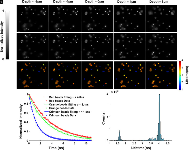
Fluorescence lifetime imaging microscopy (FLIM) is a powerful imaging technique that enables the visualization of biological samples at the molecular level by measuring the fluorescence decay rate of fluorescent probes. This provides critical information about molecular interactions, environmental changes, and localization within biological systems. However, creating high-resolution lifetime maps using conventional FLIM systems can be challenging, as it often requires extensive scanning that can significantly lengthen acquisition times. This issue is further compounded in three-dimensional (3D) imaging because it demands additional scanning along the depth axis. To tackle this challenge, we developed a computational imaging technique called light-field tomographic FLIM (LIFT-FLIM). Our approach allows for the acquisition of volumetric fluorescence lifetime images in a highly data-efficient manner, significantly reducing the number of scanning steps required compared to conventional point-scanning or line-scanning FLIM imagers. Moreover, LIFT-FLIM enables the measurement of high-dimensional data using low-dimensional detectors, which are typically low cost and feature a higher temporal bandwidth. We demonstrated LIFT-FLIM using a linear single-photon avalanche diode array on various biological systems, showcasing unparalleled single-photon detection sensitivity. Additionally, we expanded the functionality of our method to spectral FLIM and demonstrated its application in high-content multiplexed imaging of lung organoids. LIFT-FLIM has the potential to open up broad avenues in both basic and translational biomedical research.

Keywords: 3D imaging; fluorescence lifetime imaging microscopy; light field imaging.

Fig. 1.

Optical setup and image formation models. Image formation model of LIFT-FLIM (A) and LIFT-sFLIM (B). (C) System schematics. SPAD, single-photon avalanche diode; TCSPC, time-correlated single-photon counting.

Fig. 2.

Deep-learning-based image enhancement neural network. The network consists of two down- and up-sampling streams. Each stream has five ResNet blocks in both down-sampling and up-sampling paths. Each ResNet block contains four ResNet layers, and each ResNet layer has two 3 × 3 convolutional layers and one 1 × 1 convolutional layer, as indicated in the bottom right panel. Strided convolutional layers were added between the two adjacent ResNet blocks to halve the spatial dimensions in the down-sampling path, and conversely transposed strided convolutional layers were utilized to implement up-sampling in the up-sampling path. The spatial dimensions of the ResNet blocks in the sampling streams from left to right are 256 × 256, 128 × 128, 64 × 64, 32 × 32, 16 × 16, 32 × 32, 64 × 64, 128 × 128, and 256 × 256. The central 16 × 16 ResNet blocks are shared by the down- and up-sampling streams. Skip connections connect each ResNet block in the down-sampling path with its counterpart block in the up-sampling path. The inputs to the network include LIFT refocused depth image stack using filtered back projection from depth $-z_0$ to depth $z_0$, reference image captured at depth zero, and a DPM stack. The output is a high-resolution image stack at the corresponding depths. DPM: digital propagation matrix. ${\sigma }_1,{\sigma }_2$: activation functions. Conv2d: convolution 2D.

Fig. 3.

LIFT-FLIM of mixed fluorescent beads. (A) Reference intensity images at depths of −8 µm, −4 µm, 0 µm, 4 µm, and 8 µm. (B) Time-integrated LIFT-FLIM images at the corresponding depths. The refocusing to continuous depths is visualized in Movie S1. (C) Lifetime images at the corresponding depths. (D) Fluorescence decay curves at representative beads’ locations. (E) Histogram of pixel lifetimes at depth zero (Scale bar, 20 µm.) Data acquisition time: 18 s. Total number of projection angles: 45.

Fig. 4.

LIFT-FLIM of a mouse kidney tissue section. (A) Reference intensity image at depth zero. (B) Reconstructed lifetime images at depths of −8 µm, −4 µm, 0 µm, 4 µm, and 8 µm. The refocusing to continuous depths is visualized in Movie S2. (C) Fluorescence decay curves at two representative fluorophore locations. (D) Histogram of pixel lifetimes at depth zero. (E) Phasor plot. The data points were pseudocolored based on their probability of belonging to a specific cluster (red, phalloidin; green, WGA). The probability contour lines ranging from outer to inner space correspond to values of 0.1, 0.3, 0.5, 0.7, and 0.9. (F) Unmixed fluorophore image at depth zero. Red channel, phalloidin. Green channel, WGA. (G) 3D visualization of unmixed fluorophores’ distribution. Visualization from other perspective angles is provided in Movie S3. Scale bars in all figures: 20 µm. Data acquisition time: 36 s. Total number of projection angles: 90.

Fig. 5.

LIFT-FLIM of a human lung cancer pathology slide. (A) Left panel: Stitched reference intensity image. Right panel: Zoom-in image of the circled area in the Left panel. The image is blurred due to focal drift during extensive scanning. (B) Left panel: Stitched all-in-focus time-integrated LIFT-FLIm image. Right panel: Zoom-in image of the circled area in the Left panel. (C) Intensity profiles of dashed lines in A and B. (D) Stitched all-in-focus lifetime image. The lifetime image is masked with an intensity threshold (E) Zoom-in image of the circled area in D. (F) Hematoxylin and eosin (H&E)-stained image from an adjacent tissue slice. The tumor/normal tissue boundary was identified by a pathologist and annotated with a white dashed line. (G) Average pixel lifetimes in the tumor and normal tissues areas in E. The SD is shown as error bars. (H) Phasor plot. The data points were pseudocolored based on its probability belonging to a specific cluster (Red, tumor; Green, normal). The probability contour lines ranging from outer to inner space correspond to values of 0.1, 0.3, 0.5, 0.7, and 0.9. (I) Classified tissue map. Red channel, tumor; green channel, normal. Scale bars in all figures: 100 µm. The data acquisition takes 36 s for each scanned FOV. Total number of projection angles for each scanned FOV: 90.

Fig. 6.

LIFT-FLIM of lung organoids. (A) Fluorescence decay curves (Left panel) and emission spectra (Right panel) of the fluorophores used. (B–D) Reconstructed LIFT-sFLIM (B) intensity image, (C) wavelength-integrated lifetime image, and (D) time-integrated wavelength image at depth zero. (E) Lifetime phasor plot. The data points were pseudocolored based on its probability belonging to a specific cluster (red, sma, collagen, p16; green: smad3). The probability contour lines ranging from outer to inner space correspond to values of 0.2, 0.35, 0.65, and 0.95. (F) Spectral phasor plot. The data points were pseudocolored based on its probability belonging to a specific cluster (magenta: collagen, smad3; yellow: sma; green, p16). The probability contour lines ranging from outer to inner space in the magenta and yellow clusters correspond to values of 0.45, 0.65, and 0.85, while the contour lines in the green cluster correspond to values of 0.25, 0.45, 0.65, and 0.85. (G) Unmixed component images at depth zero. (H) 3D visualization of unmixed fluorophores’ distribution in the organoid. Visualization from other perspective angles is provided in Movie S4. Scale bar: 100 µm in all figures. Data acquisition time: 23 s. Total number of projection angles: 90.

References

1. Willem Borst J., Visser A. J. W. G., Fluorescence lifetime imaging microscopy in life sciences. Meas. Sci. Technol. 21, 102002 (2010).
1. Becker W., Fluorescence lifetime imaging – techniques and applications. J. Microsc. 247, 119–136 (2012). - PubMed
1. Verveer P. J., Wouters F. S., Reynolds A. R., Bastiaens P. I. H., Quantitative imaging of lateral ErbB1 receptor signal propagation in the plasma membrane. Science 290, 1567–1570 (2000). - PubMed
1. Bastiaens P. I. H., Jovin T. M., Microspectroscopic imaging tracks the intracellular processing of a signal transduction protein: Fluorescent-labeled protein kinase C βI. Proc. Natl. Acad. Sci. U.S.A. 93, 8407–8412 (1996). - PMC - PubMed
1. Sun Y., Day R. N., Periasamy A., Investigating protein-protein interactions in living cells using fluorescence lifetime imaging microscopy. Nat. Protoc. 6, 1324–1340 (2011). - PMC - PubMed