Offline hippocampal reactivation during dentate spikes supports flexible memory

Abstract

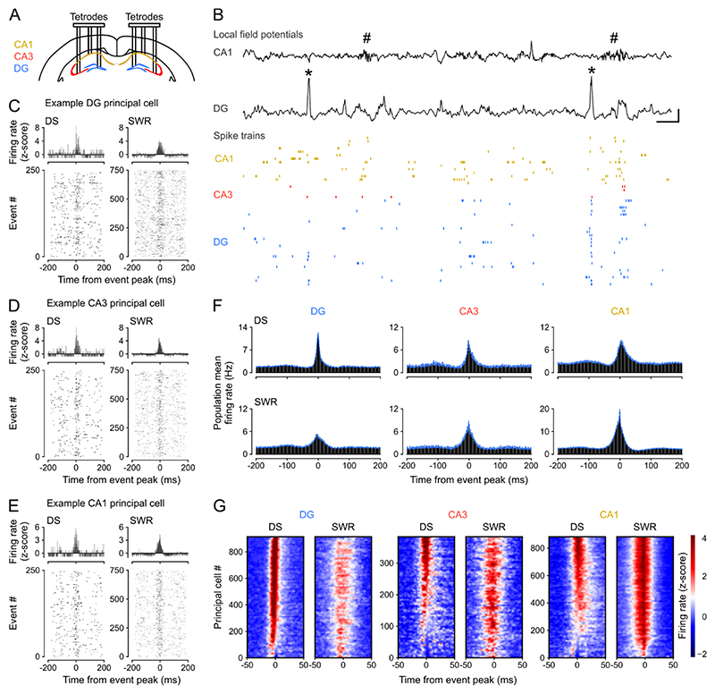
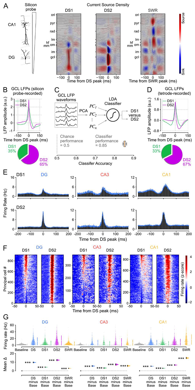
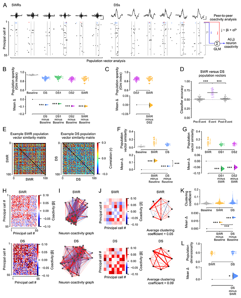
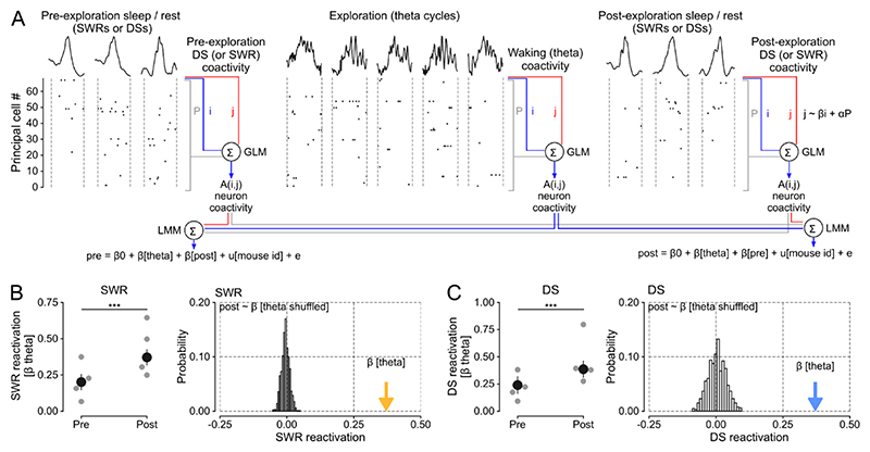
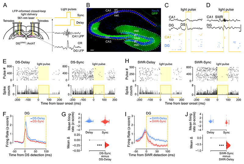
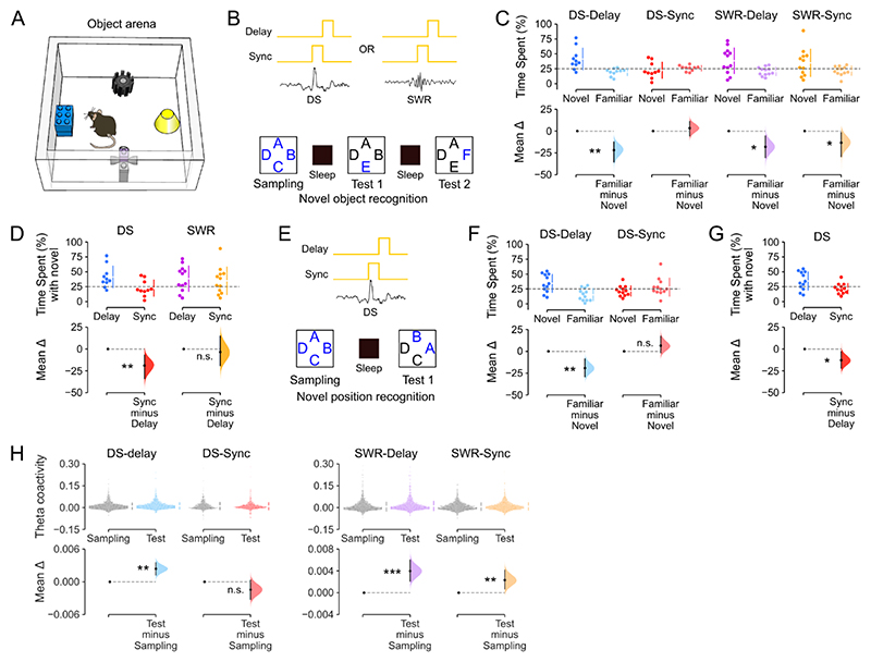
Stabilizing new memories requires coordinated neuronal spiking activity during sleep. Hippocampal sharp-wave ripples (SWRs) in the cornu ammonis (CA) region and dentate spikes (DSs) in the dentate gyrus (DG) are prime candidate network events for supporting this offline process. SWRs have been studied extensively, but the contribution of DSs remains unclear. By combining triple-ensemble (DG-CA3-CA1) recordings and closed-loop optogenetics in mice, we show that, like SWRs, DSs synchronize spiking across DG and CA principal cells to reactivate population-level patterns of neuronal coactivity expressed during prior waking experience. Notably, the population coactivity structure in DSs is more diverse and higher dimensional than that seen during SWRs. Importantly, suppressing DG granule cell spiking selectively during DSs impairs subsequent flexible memory performance during multi-object recognition tasks and associated hippocampal patterns of neuronal coactivity. We conclude that DSs constitute a second offline network event central to hippocampal population dynamics serving memory-guided behavior.

Keywords: dentate spikes; hippocampus; memory consolidation; neuronal coactivity; offline reactivation; population patterns; sharp-wave ripples.

Figure 1. Dentate spikes recruit principal cell spiking across DG, CA3, and CA1.

(A) Triple-(DG-CA3-CA1) ensemble tetrode recording allowed simultaneous monitoring of local field potentials (LFPs) and spiking activities. (B) Upper: raw wide-band CA1 and DG LFP traces (black) showing sharp-wave ripples (SWRs, hash symbols) in CA1 and dentate spikes (DSs, asterisks) in DG. Scale bars, 100 ms (horizontal), 1.5 mV for DG and 0.5 mV for CA1 (vertical). Lower: (color-coded) raster-plot of spike trains from CA1 (orange), CA3 (red), and DG (blue) principal cells (PCs, one cell per row). Shown is a few second sample of recording for clarity. (C-E) Spiking responses from single example DG (C), CA3 (D), and CA1 (E) principal cells. Upper: Z-scored peri-event time histogram (PETH) during DSs (left) and SWRs (right). Lower: corresponding raster plot showing event-related spiking responses (one event per row). (F) Group averaged firing rate PETHs for hippocampal PCs during DSs (top) and SWRs (bottom): DG (n=921), CA3 (n=388), CA1 (n=887) cells from 12 mice. Blue traces: mean ± SEM. (G) Heatmaps showing z-scored firing rates for the DG, CA3, and CA1 PCs shown in (F). For each heatmap: one cell per row, sorted (top-to-bottom) from the most activated (highest z-score at event peak, 0 ms, red) to the least activated (lowest z-score at event peak, blue) during DSs.

Figure 2. Hippocampal principal cell firing is higher in DS₂ than DS₁.

(A) Left: Laminar (64-channel) silicon-probe recording allowed simultaneous monitoring of LFPs across hippocampal layers for current source density (CSD) analysis. Right: Example (radially organized) mean LFP traces (gray) with superimposed CSD profile (heatmaps) for type 1 (DS₁) and type 2 (DS₂) dentate spikes and SWRs (calculated from 2,231 DS events and 8693 SWR events in one mouse). Note the distinct CSD profiles reflecting the different transmembrane currents associated with DS₁ versus DS₂ versus SWR events. Hippocampal layers: oriens (ori); pyramidale (pyr); radiatum (rad); lacunosum-moleculare (lm); outer (om), middle (mm), and inner (im) moleculare; granulare (gcl). Hippocampal fissure (hf). (B) Upper: Shown for silicon-probe recorded DS₁ and DS₂ identified from their CSD profiles are example average granule cell layer LFP waveforms triggered by the peak of these events. Lower: in these recordings there was a higher proportion of DS₂ than DS₁ events (n=15,067 events, 3 mice). (C) Upper: we applied principal component analysis on the normalized granule cell layer LFP waveforms for all silicon-probe recorded DS events. We then used the principal components explaining 90% of the variance to train a linear discriminant classifier with the true labels (DS₁ versus DS₂) determined by the individual CSD profiles. Lower: the classifier performance (>85%) was significantly above chance level (50%) when tested on silicon-probe recorded LFP waveforms of unlabeled events. We used this classifier to next distinguish DS₁ and DS₂ from tetrode-recorded granule cell layer LFP waveforms (D). (D) Upper: Shown for tetrode-recorded DS events are the average granule cell layer LFP waveforms for DS₁ and DS₂ predicted label obtained from the silicon-probe-based classifier (C). Lower: these recordings also contained a higher proportion of DS₂ than DS₁ events (n=32,215 events, 12 mice). (E) Group averaged firing rate PETHs for tetrode-recorded DG, CA3, CA1 principal cells during DS₁ and DS₂ (as Figure 1F,G). Blue traces: mean ± SEM. (F) Heatmaps showing z-scored firing rates for the DG, CA3, and CA1 cells shown in (E). For each heatmap: one cell per row, sorted (top-to-bottom) from the most activated (highest z-score) to least activated (lowest z-score) during DS₁ peaks. (G) Estimation plot showing the effect size for the differences in firing rate of DG, CA3, CA1 principal cells during all DS events, DS₁ and DS₂ events analyzed separately, and SWRs compared to equivalent (50 ms duration matched) baseline windows (Base) in which no DSs or SWRs occurred. Upper: raw data points (each point represents one cell), with the gapped lines on the right as mean (gap) ± s.d. (vertical ends) for each event. Lower: difference (Δ) in firing rate between Baseline windows and all DS, DS₁, DS₂, and SWR events computed from 5,000 bootstrapped resamples and with the difference-axis origin (dashed line) aligned to the baseline rate (black dot, mean; black ticks, 95% confidence interval; filled curve, sampling-error distribution). The test statistic is the mean difference, shown on the y-axis of the lower plot. P-values are from paired permutation tests, event versus baseline, ***P < 0.001. E-G show data from n=2196 hippocampal principal cells (DG: n=921, CA3: n=388, CA1: n=887) from 12 mice.

Figure 3. The coactivity structure of population spiking differs between DSs and SWRs.

(A) Analytical framework: the population-level coactivity structure was analyzed using population vectors of principal cell spiking transiently nested in individual SWRs, DSs, or duration-matched (50 ms) baseline control windows. Scale bars show 20ms and 0.5mV for SWRs and 1mv for DSs. For the analyses in panels B-G, these population firing vectors were then binarized (for each cell: a non-zero spike count gives 1; or else 0). For the analyses in H-K, we calculated the peer-to-peer coactivity, controlling for the overall population activity. (B, C) Estimation plots showing the effect size for the differences in population sparsity (using the Gini index) during DSs (with DS₁ and DS₂ plotted altogether or separately), SWRs, and compared to equivalent (50 ms duration matched) baseline windows (Baseline) in which no DSs or SWRs occurred. Upper: raw data points (each point represents one session with at least 100 of each event type and 20 principal cells), with the gapped lines on the right as mean (gap) ± s.d. (vertical ends) for each event. Lower: difference (Δ) in sparsity between Baseline windows and all DS, DS₁, DS₂, and SWR events computed from 5,000 bootstrapped resamples and with the difference-axis origin (dashed line) aligned to the baseline sparsity (black dot, mean; black ticks, 95% confidence interval; filled curve, sampling-error distribution). (C) as B but comparing population sparsity during SWR versus DS₂. Note that DS₂ and SWR events have equivalent sparsity, indicating they engage similar levels of neuronal activity. (D) A logistic regression classifier trained on population vectors nested in SWR versus DS events, or matched duration pre-event and post-event control windows, using a 4-fold cross-validation approach (75% of vectors for training; the remaining 25% for evaluation), significantly discriminated DSs from SWRs, but could not discriminate between pre-DS versus pre-SWR, and post-DS versus post-SWR vectors. Gray horizontal bars: mean classification accuracy. (E-G) DS population firing vectors are more diverse than those in SWRs. For each sleep session, we computed the similarity (Pearson correlation coefficient) for each pair of population vectors nested in either DSs, SWRs, or duration-matched baseline windows (Baseline). (E) shows example DS and SWR matrices of cross-vector similarity for one session. Cross-population vector similarity was significantly higher in SWRs compared to both DSs and control windows (F), and when compared to DS₁ and DS₂ separately (G). (H-K) DS and SWR population firing vectors exhibit distinct topology of neuronal coactivity. The coactivity between any two (i, j) neurons was measured using a GLM that quantified their short timescale (50 ms windows centered on DS or SWR peaks) firing relationship while accounting for network-level modulation reported by the remaining principal cells in the population (A). (H) This procedure returned for both DS and SWR events an adjacency matrix of β regression weights that represented the neuron pairwise coactivity structure of the population (example matrix from one session). (I) Visualization of the corresponding matrices representing DS and SWR based neuronal coactivity graphs. For clarity, (J) shows an example subset (left) for each adjacency matrices shown in (H), along with its corresponding motifs of neuronal coactivity and average clustering coefficient (right). (K) Note that DS-based graphs contained stronger triads of coactive nodes compared to both SWR graphs and control graphs constructed from duration-matched baseline windows (Baseline), as indicated by higher mean clustering coefficients. Each point in the upper plot of K represents the mean clustering coefficient for one hippocampal principal cell (n=1265 neurons, 8 mice) (L) The dimensionality of population vector matrices (number of principal components required to explain 90% of the variance) was higher for DSs than SWRs. For B-D, F-G, L: each data point shows one recording session (n=34 recording sessions from 8 mice). The test statistic is the mean difference, shown on the y-axis of each lower plot. P-values are from paired permutation tests, event versus baseline (B,F,K); event versus event (C,F,K,L); or event versus pre-event, event versus post-event (D), *P < 0.05, **P < 0.01, ***P < 0.001.

Figure 4. Waking patterns of hippocampal coactivity reactivate in offline DSs.

(A) DS and SWR reactivation of waking patterns formed by principal cell theta coactivity. For each cell pair (i, j), we predicted the spike discharge of neuron j from the activity of neuron i while regressing out the activity of the remaining population during pre-exploration sleep, exploration of open-field arenas, and post-exploration sleep (using GLMs as in Figure 3A). We separately applied this procedure for DSs and SWRs in both sleep/rest sessions (offline DS versus offline SWR coactivity), and across theta cycles in the exploration session (waking theta coactivity). This procedure returned a matrix of β regression weights that represented the neurons pairwise coactivity structure of the population in each session. We then used a Linear Mixed Model (LMM) to compare the waking theta coactivity with post-exploration sleep coactivity (in DSs or SWRs) while controlling for pre-exploration sleep coactivity (in DSs or SWRs), and vice versa (reverse model). We included mouse identity as a random factor in each LMM. (B) SWR reactivation (measured by the β coefficients of the LMM that predicted post-exploration SWR coactivity from waking theta coactivity, controlling for pre-exploration SWR coactivity). Left: The β coefficient for theta coactivity was significantly higher when predicting post-exploration SWR coactivity than with the reverse model (i.e., predicting pre-exploration SWR coactivity from theta coactivity, controlling for post-exploration SWR coactivity). Gray points show the β coefficient for theta coactivity for individual mice. Error bars show ± 95% confidence interval. P-value from t-test comparing post versus pre β coefficients: t(7308) = 10.29; P < 0.0001. Right: The histogram shows the random probability distribution of β weights for theta coactivity when cell pair identity was shuffled (i.e., a null distribution based on 1,000 random shuffles; n=7,310 cell pairs from 4 mice). The colored arrow shows the actual β coefficient for theta coactivity. (C) DS reactivation exhibited the same pattern of results as SWR reactivation, shown in B. P-value from t-test comparing post versus pre β coefficients t(7308) = 8.84; P < 0.0001.

Figure 5. DS- and SWR-informed offline suppressions of DG granule cell activity.

(A) Triple-(DG-CA3-CA1) ensemble recording with LFP-informed yellow (561 nm) DG light-delivery. Dentate granule cells (DGCs) transduced with ArchT-GFP (DG^Grm2::ArchT). Closed-loop light-delivery to suppress DGC spiking immediately upon either DS detection (DS-Sync condition) or SWR detection (SWR-Sync) or their respective control conditions (DS-Delay and SWR-Delay, where light delivery was offset by 100 ms after event detection). (B) ArchT-GFP-expressing DGCs in a DG^Grm2::ArchT mouse. Neuronal nuclei stained with NeuN. Scale bar=100 μm. Granule cell layer: gcl; molecular layer: mol; pyramidal cell layer: pyr; stratum oriens: ori; radiatum: rad; lucidum: s.l. (C, D) Closed-loop feedback transiently silenced DGCs during either DG DS (C; “DS-Sync”) or CA1 SWR (D; “SWR-Sync”) events, illustrated with raw data examples. Scale bars, 30 ms (horizontal), 1.5 mV (vertical). (E) Raster plots (event-related spiking response; one light pulse per row (Upper), and peri-event time histograms (Lower) showing photo-silencing of two example DG cells from a DG^Grm2::ArchT mouse in DS-Delay and DS-Sync. (F, G) Corresponding quantification of average DGC firing rate (z-score) for DS-Delay versus DS-Sync (F,G; n=548 cells in 9 mice). In F, the orange box shows the laser-on period for DS-Sync. (H-J) As E-G but showing DGC photo-silencing during SWR-Delay and SWR-Sync conditions (I, J; n=181 cells in 3 mice). In I, the orange box shows the laser-on period for SWR-Sync. For G and J, the test statistic is the mean difference, shown on the y-axis of each lower plot. P-values are from unpaired permutation tests, Delay versus Sync, ***P < 0.001.

Figure 6. Offline suppression of DS activity impairs flexible recognition memory.

(A) Behavioral arena used for the recognition memory tasks. (B-D) Offline DS events are required for novel object recognition memory. (B) Task layout. During sleep sessions (interposed between novel object exploration sessions), closed-loop optogenetic suppression of DG cells in DG^Grm2::ArchT mice was achieved using real-time monitoring of either DG or CA1 LFPs to actuate either DS synchronized (DS-Sync) or delayed (DS-Delay), SWR synchronized (SWR-Sync) or delayed (SWR-Delay) DG light delivery. Letters depict object locations in the task arena (A), with novel objects in blue. (C) Estimation plot showing the percentage of time spent by mice with the novel versus the familiar objects in each of the four LFP-informed closed-loop conditions. Upper: Each data point represents the percentage time spent with the novel object versus the mean percentage time spent with the three familiar objects; chance performance is shown by the dashed line. Lower: mean difference between novel and familiar object exploration time. (D) as C but directly comparing novel object preference in the delay versus sync conditions for DS and SWR events. Mice in the DS-Delay, SWR-Delay, and SWR-Sync conditions, but not the DS-Sync condition, exhibited a significant preference for novel over familiar objects (DS-Delay and DS-Sync: n=10 sessions, in 3 mice; SWR-Delay and SWR-Sync: n=12 sessions in 3 mice). (E-G) Likewise, offline DS events are required for novel position recognition memory. (E) Task layout. Letters depict object locations, with novel positions in blue. (F) Estimation plot showing the percentage of time spent by DG^Grm2::ArchT mice with the novel versus the familiar object locations following sleep sessions with DS-Sync or DS-Delay suppression of DG cells. Upper: Each data point represents the percentage time spent with objects in novel locations versus objects in familiar locations; chance performance is shown by the dashed line. Lower: mean difference between novel and familiar location exploration times. (G) As F but directly comparing novel location preference in DS-Delay versus DS-Sync. Mice in the DS-Delay but not the DS-Sync condition exhibited a significant preference for objects in novel over familiar locations (n=12 novel versus n=12 familiar locations, 6 sessions, in 4 mice). (H) In the object recognition task, the theta peer-to-peer coactivity increased from the initial object sampling to the memory test following offline DG cell suppression in the DS-Delay, SWR-Delay, and SWR-Sync conditions; but this was not the case in the DS-sync condition (where mice exhibited no novel object preference). Paired estimation plot showing theta coactivity during Sampling versus Test. Upper: each point represents a beta coefficient for the theta-nested peer-to-peer coactivity between pairs of hippocampal principal cells (n=1537, n=678, n=1719, n=1482 cell pairs, respectively, in 6 mice). Lower: black dot, mean difference between sampling and test sessions; black ticks, 95% confidence interval. For C,D and F-H, the test statistic is the mean difference, shown on the y-axis of each lower plot. P-values are from paired permutation tests, Familiar versus Novel (C,F); Delay versus Sync (D,G); or Test versus Sampling (H), *P < 0.05, **P < 0.01, ***P < 0.001.

References

1. Maquet P. The Role of Sleep in Learning and Memory. Science. 2001;294:1048–1052. - PubMed
1. Walker MP, Stickgold R. Sleep, Memory, and Plasticity. Annual Review of Psychology. 2006;57:139–166. - PubMed
1. Klinzing JG, Niethard N, Born J. Mechanisms of systems memory consolidation during sleep. Nat Neurosci. 2019;22:1598–1610. - PubMed
1. Brodt S, Inostroza M, Niethard N, Born J. Sleep—A brain-state serving systems memory consolidation. Neuron. 2023;111:1050–1075. - PubMed
1. Buzsáki G. Neural Syntax: Cell Assemblies, Synapsembles, and Readers. Neuron. 2010;68:362–385. doi: 10.1016/j.neuron.2010.09.023. - DOI - PMC - PubMed
LinkOut - more resources