Task-Adaptive Angle Selection for Computed Tomography-Based Defect Detection

Abstract

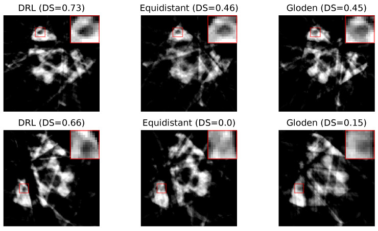
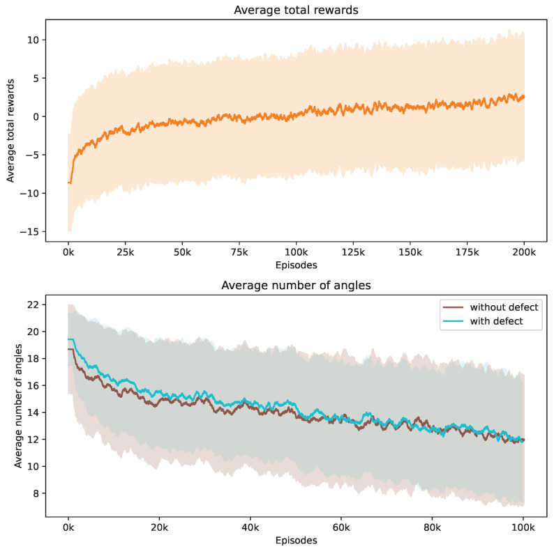
Sparse-angle X-ray Computed Tomography (CT) plays a vital role in industrial quality control but leads to an inherent trade-off between scan time and reconstruction quality. Adaptive angle selection strategies try to improve upon this based on the idea that the geometry of the object under investigation leads to an uneven distribution of the information content over the projection angles. Deep Reinforcement Learning (DRL) has emerged as an effective approach for adaptive angle selection in X-ray CT. While previous studies focused on optimizing generic image quality measures using a fixed number of angles, our work extends them by considering a specific downstream task, namely image-based defect detection, and introducing flexibility in the number of angles used. By leveraging prior knowledge about typical defect characteristics, our task-adaptive angle selection method, adaptable in terms of angle count, enables easy detection of defects in the reconstructed images.

Keywords: adaptive angle selection; computed tomography; deep learning; defect detection; reinforcement learning.

Figure 1

The DRL network selects the next angle ${\theta }_{i+1}$, which is used, along with the previously selected ones and measurements, to gather a new reconstruction. The SSIM is then calculated to assess the similarity between this reconstruction and the ground truth image. Concurrently, the contrast ratio value is derived from the ground truth of the defect (indicated by the dashed line); alternatively, the Dice score value is determined by comparing the defect segmentation output with the defect’s ground truth (depicted by the solid line). These metrics inform the DRL network’s decision-making for further angle selection.

Figure 2

This figure displays samples of Shepp–Logan shapes, illustrating both normal (top row) and defective variants (bottom row). Each sample is unique, demonstrating a range of scales, shifts, and rotations, which reflects the diversity of the dataset used in our analysis.

Figure 3

Evolution of average total rewards and the number of angles over training episodes. The figure at the top presents the trend in average total rewards achieved by the DRL agent throughout the training episodes. The figure at the bottom illustrates the variation in the average number of angles selected by the DRL agent for Shepp–Logan shapes, differentiated by the presence or absence of defects. Analyzed at intervals of every 1000 episodes, the graph shows mean values as a central curve, signifying the average reward at each point, with variance depicted as shaded bands around the curve, representing the standard deviation and the spread of reward values over time.

Figure 4

Reconstruction quality comparison. This figure presents a side-by-side comparison of reconstructed images obtained using the DRL policy versus those acquired through the equidistant and golden standard policies. The comparison highlights the differences in defect visibility across these methodologies. The numerical value accompanying each title denotes the CR value pertinent to its respective image, serving as a quantitative measure of the defect contrast compared to its surroundings. Red rectangles highlight the defect in each image, with a zoomed-in view displayed in the upper right corner to facilitate a more detailed examination of the defect visibility.

Figure 5

This figure presents a side-by-side comparison of CR values derived from different imaging policies. It specifically highlights the differences in CR values achieved by the DRL policy that utilizes both SSIM and CR as rewards, in contrast to the equidistant and golden standard policies. The number of angles selected by the DRL policy, which integrates SSIM and CR rewards, forms the basis for this comparison. The DRL policy informed by SSIM alone selects a smaller number of angles. It takes into account 1000 episodes, with the mean values representing the average. Additionally, calculations not depicted in this figure indicate that the DRL policy exhibits the smallest variance among these policies once the mean values reach a point of convergence.

Figure 6

The top row depicts the selected ROI from the initial dataset, devoid of any defects. The bottom row presents three samples with artificially inserted pore defects within the ROI, each sample exhibiting a unique combination of rotation and scale variations to simulate defect diversity.

Figure 7

The top row depicts the selected ROI from the initial dataset, devoid of any defects. The bottom row presents three samples with artificially inserted crack defects within the ROI, each sample exhibiting a unique combination of rotation and scale variations to simulate defect diversity.

Figure 8

Evolution of average total rewards and the number of angles over training episodes. The figure at the top presents the trend in average total rewards achieved by the DRL agent throughout the training episodes. The figure at the bottom illustrates the variation in the average number of angles selected by the DRL agent for samples with ROI 1, differentiated by the presence or absence of defects. Analyzed at intervals of every 1000 episodes, the graph shows mean values as a central curve, signifying the average reward at each point, with variance depicted as shaded bands around the curve, representing the standard deviation and the spread of reward values over time.

Figure 9

Reconstruction quality comparison. This figure presents a side-by-side comparison of reconstructed images obtained using the DRL policy versus those acquired through the equidistant and golden standard policies. The comparison highlights the differences in defect visibility across these methodologies. The numerical value accompanying each title denotes the DS value pertinent to its respective image, serving as a quantitative measure of the defect segmentation. Red rectangles highlight the defect in each image, with a zoomed-in view displayed in the upper right corner to facilitate a more detailed examination of the defect visibility.

Figure 10

Comparative analysis of the pore defect segmentation. The top row represents the original image with ground truth defects. The middle row illustrates segmentation outputs using three different policies: DRL policy, equidistant policy, and a golden standard policy. The bottom row displays the corresponding defect masks generated by K-means clustering. The values of the DS for each method are indicated, quantifying the accuracy of the defect segmentation relative to the ground truth.

Figure 11

This figure presents a side-by-side comparison of DS values derived from different imaging policies. It specifically highlights the differences in DS values achieved by the DRL policy that utilizes both SSIM and DS as rewards, in contrast to the equidistant and golden standard policies. The number of angles selected by the DRL policy, which integrates SSIM and DS rewards, forms the basis for this comparison. The DRL policy informed by SSIM alone selects a smaller number of angles. It takes into account 1000 episodes, with the mean values representing the average. Additionally, calculations not depicted in this figure indicate that the DRL policy exhibits the smallest variance among these policies once the mean values reach a point of convergence.

Figure 12

Evolution of average total rewards and the number of angles over training episodes. The figure at the top presents the trend in average total rewards achieved by the DRL agent throughout the training episodes. The figure at the bottom illustrates the variation in the average number of angles selected by the DRL agent for samples with ROI 2, differentiated by the presence or absence of defects. Analyzed at intervals of every 1000 episodes, the graph shows mean values as a central curve, signifying the average reward at each point, with variance depicted as shaded bands around the curve, representing the standard deviation and the spread of reward values over time.

Figure 13

Reconstruction quality comparison. This figure presents a side-by-side comparison of reconstructed images obtained using the DRL policy versus those acquired through the equidistant and golden policies. The comparison highlights the differences in defect visibility across these methodologies. The numerical value accompanying each title denotes the DS value pertinent to its respective image, serving as a quantitative measure of the defect segmentation. Red rectangles highlight the defect in each image, with a zoomed-in view displayed in the upper right corner to facilitate a more detailed examination of the defect visibility.

Figure 14

Comparative analysis of the crack defect segmentation. The top row represents the original image with ground truth defects. The middle row illustrates segmentation outputs using three different policies: DRL policy, equidistant policy, and a golden standard policy. The bottom row displays the corresponding defect masks generated by K-means clustering. The values of the Dice score for each method are indicated, quantifying the accuracy of the defect segmentation relative to the ground truth.

Figure 15

This figure presents a side-by-side comparison of DS values derived from different imaging policies. It specifically highlights the differences in DS values achieved by the DRL policy that utilizes both SSIM and DS as rewards, in contrast to the equidistant and golden standard policies. The number of angles selected by the DRL policy, which integrates SSIM and DS rewards, forms the basis for this comparison. The DRL policy informed by SSIM alone selects a smaller number of angles. It takes into account 1000 episodes, with the mean values representing the average. Additionally, calculations not depicted in this figure indicate that the DRL policy exhibits the smallest variance among these policies once the mean values reach a point of convergence.

References

1. Kazantsev I. Information content of projections. Inverse Probl. 1991;7:887. doi: 10.1088/0266-5611/7/6/010. - DOI
1. Fischer A., Lasser T., Schrapp M., Stephan J., Noël P.B. Object specific trajectory optimization for industrial X-ray computed tomography. Sci. Rep. 2016;6:19135. - PMC - PubMed
1. Batenburg K.J., Palenstijn W.J., Balázs P., Sijbers J. Dynamic angle selection in binary tomography. Comput. Vis. Image Underst. 2013;117:306–318.
1. Dabravolski A., Batenburg K.J., Sijbers J. Dynamic angle selection in X-ray computed tomography. Nucl. Instruments Methods Phys. Res. Sect. B Beam Interact. Mater. Atoms. 2014;324:17–24.
1. Burger M., Hauptmann A., Helin T., Hyvönen N., Puska J.P. Sequentially optimized projections in X-ray imaging. Inverse Probl. 2021;37:075006.
LinkOut - more resources