The representation of decision variables in orbitofrontal cortex is longitudinally stable

Abstract

The computation and comparison of subjective values underlying economic choices rely on the orbitofrontal cortex (OFC). In this area, distinct groups of neurons encode the value of individual options, the binary choice outcome, and the chosen value. These variables capture both the choice input and the choice output, suggesting that the cell groups found in the OFC constitute the building blocks of a decision circuit. Here, we show that this neural circuit is longitudinally stable. Using two-photon calcium imaging, we record from the OFC of mice engaged in a juice-choice task. Imaging of individual cells continues for up to 40 weeks. For each cell and each session pair, we compare activity profiles using cosine similarity, and we assess whether the neuron encodes the same variable in both sessions. We find a high degree of stability and a modest representational drift. Quantitative estimates indicate that this drift would not randomize the circuit within the animal's lifetime.

Keywords: Neuroscience; calcium imaging; decision circuit; decision making; economic choice; longitudinal stability; orbitofrontal cortex; representational drift; subjective value; two-photon microscopy.

Figure 1.. Choice task and behavioral performance

(A) Experimental apparatus. The animal was head fixed under the microscope objective. Two odors, each representing one of two offered juices, were presented simultaneously from the left and right. The mouse indicated its choice by licking one of two spouts. (B) Trial structure. Following an inter-trial interval (ITI; 2.5–5 s), odors were delivered from the two odor ports. The offer period lasted 2.4 s and ended with an acoustic tone (0.2 s; go signal). The animal indicated its choice within 5 s. Immediately after the first lick following the go signal, the corresponding juice was delivered. During the subsequent ITI, a vacuum system removed all remaining odors from the field. (C) Example sessions and choice patterns. In each plot, offer types are represented on the x axis. The y axis indicates the percentage of trials in which the animal chose juice B. Sigmoid curves were obtained from logistic regressions. Relative value $(\rho )$, choice accuracy $(\eta )$, and side bias $(\epsilon )$ are indicated for each session. (D–F) Population histograms for behavioral parameters. In (F), the dashed lines highlight $\mid \epsilon \mid =0.5$ and $\mid \epsilon \mid =1$ (see STAR Methods).

Figure 2.. Longitudinal analysis of choice accuracy

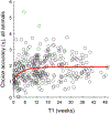
We pooled 343 sessions from 13 mice (entire dataset). Each circle represents one session, and the red line was obtained from an exponential fit. Two outliers (green circles) were excluded from the fit. Referring to Equation 3, the fitted parameters (95% confidence interval) were $a=-0.75(-1.03,-0.46)$, $b=0.03(0.005,0.06)$, and $c=1.90(1.78,2.02)$. Thus, the behavioral performance, quantified by choice accuracy $\eta$, improved significantly as mice became more expert in the task.

Figure 3.. Longitudinal two-photon imaging of OFC

(A) Viral expression and lens location. Left: coronal slice (anterior-posterior = +2.65 mm) obtained from a mouse 2 months after a surgery in which we injected AAV-Syn-GCaMP6f in the OFC and implanted a 1 mm diameter GRIN lens. Cell nuclei were stained by DAPI (white), and cells expressing GCaMP6f are contained in the green injection site. The location of the GRIN lens is clearly visible. The borders of OFC are highlighted (white dotted line) by matching them with a coronal section obtained from the Allen Brain Atlas (2011; right). The focal plane (red dotted line) was calculated based on the lens working distance. (B) Example FOV. Imaging segmentation revealed the presence of n = 169 cells. White contours show neuronal locations. Red contours show 12 example cells illustrated in (C). A, anterior; M, medial. Scale bar, 100 μm. (C) $\Delta \mathsf{F}∕\mathsf{F}$ traces (one trial) of 12 example neurons (numbered top to bottom). Vertical lines indicate different behavioral events. Red/blue dots indicate left/right licks. (D1–D5) Example FOV recorded in five sessions over 83 days. Images remained remarkably stable throughout the recordings. Scale bar, 100 μm. (E1 and E2) Images for days 1 and 11 obtained after cell segmentation and cell matching. Orange contours indicate matching cells (n = 98 cells). White contours indicate unshared cells (n = 63 cells for day 1; n = 33 cells for day 11). (F) Longitudinal stability. We recorded 18 sessions from one single FOV over 100 days. The image illustrates the fraction of shared cells (number of shared cells/mean of cell numbers between FOVs) for every pair of sessions as a function of the time distance.

Figure 4.. CS analysis

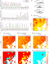
(A) Example cell. We examined the cell activity in two sessions (days 31 and 75). Single-trial traces were obtained by joining two time windows aligned with the offer onset and the time of first lick. In each session, we averaged traces over trials for each trial type, and we concatenated the mean traces obtained for different trial types. The resulting signal is referred to as the activity profile. We repeated this operation for both sessions, and we computed the cosine similarity (CS) between the two activity profiles. Here, activity profiles recorded in sessions 1 and 2 are shown in green and pink, respectively. Gray dashed lines separate trial types. Details about the trial types are indicated below the x axis: numbers indicate offered quantities $(q_B:q_A)$; diamonds and circles indicate that the animal chose juice A and juice B, respectively; and red and blue indicate that the animal chose left and right, respectively. For this neuron, CS = 0.96. (B) Example cell recorded on days 122 and 129 (CS = 0.94). (C) Example cell recorded on days 1 and 63 (CS = 0.90). (D) Distribution of CS for the three treatments (same cells, mismatched cells, shuffled times). Here, T1 = weeks 5–6, $\Delta \mathsf{T}=\mathsf{weeks}7-8$, and n = 747 cells. For each distribution, the orange vertical line indicates the median. We measured $\mathsf{median}({\mathsf{CS}}_{\text{same}})=0.677$, $\mathsf{median}({\mathsf{CS}}_{\text{mismatched}})=0.617$, and $\mathsf{median}({\mathsf{CS}}_{\text{shuffled}})=0.616$. The median measured for the ${\mathsf{CS}}_{\mathsf{same}}$ distribution is significantly higher than that measured for the ${\mathsf{CS}}_{\mathsf{mismatched}}$ distribution (p = 2.26 × 10⁻³⁸, Kruskal-Wallis test) and that measured for the ${\mathsf{CS}}_{\mathsf{shuffled}}$ distribution (p = 1.37 × 10⁻²⁹, Kruskal-Wallis test). (E) Number of cells matched across sessions as a function of T1 and $\Delta \mathsf{T}$. Session pairs were divided in bins of 2 × 2 weeks. Here, the number of cells available in each bin are illustrated with a heatmap (see color legend). Each entry in the table indicates the number of cells recorded with the corresponding T1 (x axis) and $\Delta \mathsf{T}$ (y axis). Bins with ≤ 10 cells were removed from this figure. (F–H) Measures of median(CS) as a function of T1 and $\Delta \mathsf{T}$ same cells, mismatched cells, and shuffled times. In each image, median(CS) is illustrated with a heatmap. The black dashed rectangle highlights the bin illustrated in (D). (I–K) Statistical comparison of different treatments. (I) illustrates the p values obtained comparing the distributions of CSs measured for “same cells” and “mismatched cells” treatments. (J) and (K) are for the other two comparisons. All p values (see color bar) are from a Kruskal-Wallis test.

Figure 5.. Longitudinal trends of cosine similarity

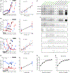
(A) Median(CS) as a function of T1 and $\Delta \mathsf{T}$ (same as Figure 4F); 6 × 6 week Bins used for longitudinal comparisons are highlighted. Median(CS) was significantly higher in Bin 2 than in Bin 1 (p = 1.55 × 10⁻¹¹⁵) and significantly lower in Bin 3 than Bin 1 (p = 0.05, Kruskal-Wallis test). (B) CS decreases with time passage $(\Delta \mathsf{T})$. To have comparable numbers of cells for different values of $\Delta \mathsf{T}$, we restricted this analysis to pairs of sessions with $\mathsf{T}1\le 6$ weeks. For each day, we computed median(CS). Here, the radius of each circle is proportional to the number of cells. We fitted data with a drift model $\mathsf{CS}(\Delta \mathsf{T})=a_0+a_1{\Delta \mathsf{T}}^{1∕2}$ (weighing data points by the number of cells) and obtained $a_0=0.6835$ and $a_1=-1.697{10}^{-3}{\text{day}}^{-1∕2}$. Red dashed lines indicate the 95% confidence interval. For the same population, we also computed $b=\mathsf{median}({\mathsf{CS}}_{\text{mismatched cells}})=0.622821$ (green dashed line). Thus, we estimated the time necessary for full reorganization, $\Delta {\mathsf{T}}_{\mathsf{FR}}=1,278$ days. (C) CS increases with task experience (T1). This analysis was restricted to pairs of sessions with $\Delta \mathsf{T}\le 6$ weeks. The red line was obtained from the fit $\mathsf{CS}(\mathsf{T}1)=a_0+a_1\mathsf{T}{1}^{1∕2}$. The green dashed line indicates the median(CS) obtained for mismatching cells. (D) CS and choice accuracy (population). Each dot represents one session, and the line was derived from a linear regression (p = 0.04). The color of the dot represents T3 (see color bar). In the inset, dots represent 25-day bins, and colors indicate T3. (E) CS, choice accuracy, and experience in the task (individual animals). Axes represent T3 (x axis) and variable X (y axis), and each data point represents one session. Different colors indicate different animals, and solid lines were derived from an ANCOVA (independent lines). For 11 of 12 animals, the two measures were positively correlated.

Figure 6.. Decision variables encoded in OFC

(A) Example cell encoding the offer value B. Left: offer types are ordered by the quantity ratio $q_B∕q_A$ (x axis). Black dots represent the choice pattern. Color symbols represent the neuronal activity $(\Delta \mathsf{F}∕\mathsf{F})$. Diamonds and circles are for trials in which the animal chose juice A and juice B, respectively. Red and blue are for trials in which the animal chose the offer on the left and right, respectively. Right: the same neuronal response is plotted against the binary variable offer value B. The cell activity increased as a function of $q_B$. The dark gray line was obtained from a linear regression. (B) Example cell encoding the position of A. The activity of this cell was roughly binary—low and high when juice A was offered on the left and right, respectively. (C and D) Example cells encoding the chosen value and the chosen side. Neuronal responses illustrated here are from (A) late delay, (B) late delay, (C) post-juice, and (D) pre-juice time windows. All conventions are as in (A). (E) Population analysis. Each response passing the ANOVA criterion was regressed against each of the 12 variables. The images illustrates for each time window (row) the number of responses best explained by each variable (column). Here, numbers and shades of gray indicate cell counts. (F) Variable selection and stepwise procedure. The top image is the same as in (E). In the first iteration, we identified the variable that explained the highest number of responses (chosen side). We removed from the pool all the responses explained by that variable (35.73% of the total). The residual pool is illustrated in the second image. The procedure was then repeated. At each iteration, we identified the variable that explained the largest number of responses in the residual pool (highlighted by a green asterisk). If the marginal explanatory power was ≥2%, then we retained the variable and removed from the pool all the responses explained by that variable. The procedure continued until all newly selected variables failed the 2% criterion. (G) Percentage of explained responses and stepwise procedure. The x axis indicates the number of variables (iterations). On the y axis, 100% corresponds to the number of responses passing the ANOVA criterion; the dotted line corresponds to the number of responses collectively explained by the 12 variables included in the analysis. (H) Percentage of explained response and best-subset procedure. The same format as in (G) is used. In (E), variables selected by both the stepwise and best-subset procedures are highlighted in green.

Figure 7.. The encoding of decision variables is longitudinally stable

(A) Contingency table (n = 649 cells). Rows and columns represent the variables encoded in sessions 1 and 2, respectively; entries and gray shades are cell counts. (B) Odds ratios (ORs). For each entry, Fisher’s exact test assessed whether the departure from chance (OR = 1) was statistically significant. Pink and blue asterisks indicate that the cell count was significantly above and below chance, respectively (*p < 0.05, **p < 0.01, and ***p < 0.001).

References

1. Gardner MPH, Sanchez D, Conroy JC, Wikenheiser AM, Zhou J, and Schoenbaum G (2020). Processing in lateral orbitofrontal cortex is required to estimate subjective preference during initial, but not established, economic choice. Neuron 108, 526–537.e4. 10.1016/j.neuron.2020.08.010. - DOI - PMC - PubMed
1. Kuwabara M, Kang N, Holy TE, and Padoa-Schioppa C (2020). Neural mechanisms of economic choices in mice. Elife 9, e49669. 10.7554/eLife.49669. - DOI - PMC - PubMed
1. Gore F, Hernandez M, Ramakrishnan C, Crow AK, Malenka RC, and Deisseroth K (2023). Orbitofrontal cortex control of striatum leads economic decision-making. Nat. Neurosci 26, 1566–1574. 10.1038/s41593-023-01409-1. - DOI - PMC - PubMed
1. Yu LQ, Dana J, and Kable JW (2022). Individuals with ventromedial frontal damage display unstable but transitive preferences during decision making. Nat. Commun 13, 4758. 10.1038/s41467-022-32511-w. - DOI - PMC - PubMed
1. Ballesta S, Shi W, Conen KE, and Padoa-Schioppa C (2020). Values encoded in orbitofrontal cortex are causally related to economic choices. Nature 588, 450–453. 10.1038/s41586-020-2880-x. - DOI - PMC - PubMed
Publication types
LinkOut - more resources