Integrative taxonomy clarifies the evolution of a cryptic primate clade

Abstract

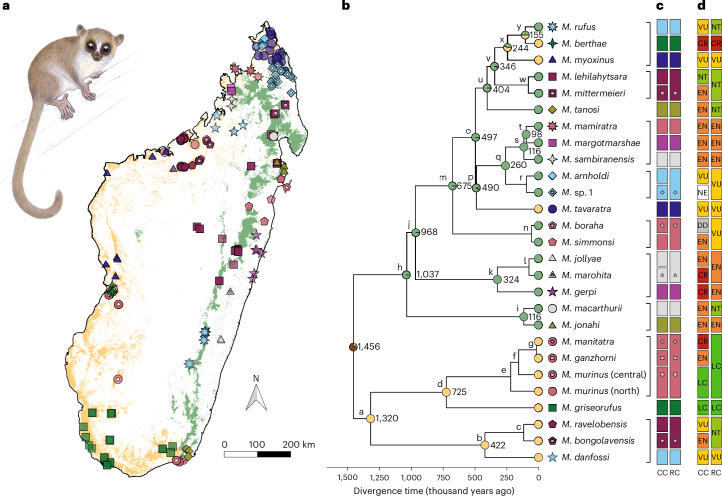
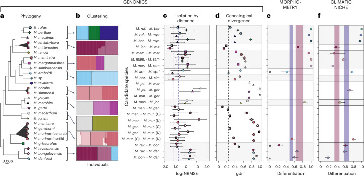
Global biodiversity is under accelerating threats, and species are succumbing to extinction before being described. Madagascar's biota represents an extreme example of this scenario, with the added complication that much of its endemic biodiversity is cryptic. Here we illustrate best practices for clarifying cryptic diversification processes by presenting an integrative framework that leverages multiple lines of evidence and taxon-informed cut-offs for species delimitation, while placing special emphasis on identifying patterns of isolation by distance. We systematically apply this framework to an entire taxonomically controversial primate clade, the mouse lemurs (genus Microcebus, family Cheirogaleidae). We demonstrate that species diversity has been overestimated primarily due to the interpretation of geographic variation as speciation, potentially biasing inference of the underlying processes of evolutionary diversification. Following a revised classification, we find that crypsis within the genus is best explained by a model of morphological stasis imposed by stabilizing selection and a neutral process of niche diversification. Finally, by clarifying species limits and defining evolutionarily significant units, we provide new conservation priorities, bridging fundamental and applied objectives in a generalizable framework.

Fig. 1. Workflow for integrative taxonomy of cryptic taxa and its illustration in the genus Microcebus.

We first test whether genetic distances between candidates clearly reject or conform to an intraspecific model of isolation by distance, using a heuristic based on normalized root mean square error (NRMSE) distributions. If neither is the case, we test whether pairs of sister candidates are reciprocally monophyletic, form distinct genetic clusters and exhibit a genealogical divergence index (gdi) above or equal to 0.2. Failure to pass one of these criteria is sufficient to reject status as distinct species. If tests are passed, we explore whether candidates exhibit substantial differentiation in at least one other taxonomic character (morphometry, climatic niche, reproductive activity, acoustic communication) that cannot be attributed to ecological flexibility, plasticity or similar factors (indicated by asterisks). If so, and only then, candidate species are confirmed. Three examples of pairs of candidate species in the genus Microcebus are presented to illustrate the workflow. Red arrows indicate the delimitation procedure. Additional taxonomic characters are not restricted to the examples given here. Brown boxes indicate which tests consider spatial variation. In principle, other taxonomic characters would benefit from being analysed in a spatial context as well. Details on how tests were conducted and differentiation was quantified can be found in the Methods.

Fig. 2. Island-wide taxogenomics of the cryptic Microcebus radiation.

a, Map of genotyped Microcebus species (symbols correspond to b). Dry and humid forests are represented in yellow and green, respectively. Illustration represents M. jonahi (illustration copyright Stephen D. Nash; used with permission). b, Microcebus phylogeny with divergence times and ancestral habitats (node pies; yellow, dry; green, humid; brown, dry and humid). Candidate groups to which our delimitation framework was applied are indicated by black brackets. White centres in species symbols represent synonymized candidates following the revised classification shown in c. Divergence times among synonymized candidates are not reported. Nodes are labelled by lowercase letters for reference to downstream analyses. c, Comparison of the current (CC, 25 described and one putative species) and revised (RC; 19 species) Microcebus classification. d, Recommended changes in International Union for Conservation of Nature (IUCN) species conservation status after taxonomic revision (NE, not valuated; DD, data deficient; LC, least concern; NT, near threatened; VU, vulnerable; EN, endangered; CR, critically endangered).

Fig. 3. Summary of species delimitation analyses in the genus Microcebus.

a, Maximum likelihood phylogeny with non-monophyly indicated by triangles. Scale is substitutions per site. b, Admixture proportions (y axis), where the number of a priori clusters K equals the number of candidate species; candidate species are separated by black bars and ordered as in a. c, NRMSE distributions of isolation by distance (log scale) with 0.05 and 0.95 quantiles; symbols indicate focal taxon for calculation of within-candidate IBD; red, pink and blue dashed lines indicate 0.95 quantiles of NRMSE distributions based on IBD within M. lehilahytsara, M. mittermeieri and continuous M. tavaratra populations, respectively (Methods). d, Genealogical divergence index (gdi) with 95% highest posterior density interval based on a coalescent model of 6,000 loci and two individuals per species (one individual for M. marohita); symbols refer to a and indicate which taxon’s θ was used for estimation; taxon names refer to the first three letters of the candidate species epithet; the dashed line indicates threshold below which candidates are considered synonyms. e, Morphometric differentiation (1 − maximum hypervolume overlap) and 95% confidence intervals (CI); asterisks indicate fit to a model of intraspecific character variation, precluding the interpretation of the differentiation signal (Supplementary Table 5). f, Climatic niche differentiation (1 − D and 95% CIs. In e and f, red and blue areas represent 95% CIs of differentiation between M. lehilahytsara and M. mittermeieri and among fragmented M. tavaratra populations, respectively. Empty rows indicate a lack of data. Sample sizes per species for c, e and f are given in Supplementary Tables 2, 4 and 6, respectively.

Fig. 4. Evolution of morphometry and climatic niche in the genus Microcebus.

a,b, Regression (dashed line) of morphometric (a) and climatic niche hypervolume (b) overlap through time, that is, across nodes of the tree in Fig. 2b. The vertical line of node b estimate represents the 95% confidence interval. Light lines represent linear regressions of 1,000 datasets simulated under the most likely models (Ornstein–Uhlenbeck (OU) for morphology and Brownian motion (BM) for climatic niche). c, Distributions of Spearman’s correlation coefficient (r_s) between node age and morphometric or climatic niche hypervolume overlap, from 1,000 simulations under OU, BM and EB models of character evolution. Dashed horizontal lines indicate the observed r_s.

Extended Data Fig. 1. Statistical test to distinguish intra- from interspecific divergence for two candidate species based on patterns of isolation by distance.

a, SNP data are divided into windows comprising 1,000 SNPs. b, For each window, individual geographic distances are correlated with genetic distances and classified as distances among candidate 1 individuals (blue), among candidate 2 individuals (yellow) or between individuals of the two candidates (green). c, Deviations of observed genetic distances between candidates from those predicted by the within-candidate geographic clines in genetic distance are calculated. Accordingly, two normalized root mean square error (NRMSE) values are obtained for each genomic window j, one for each candidate i, resulting in two NRMSE distributions across genomic windows. d, The resulting distributions are compared to the 0.95 quantiles of reference distributions (taken from M. tavaratra and M. lehilahytsara in this work). The intraspecific clinal variation model is rejected if the 0.05 quantiles of both NRMSE distributions of a candidate pair are above the 0.95 quantiles of the reference distributions, indicating that genetic distances between candidates cannot be explained by a geographic cline. Conversely, if the 0.95 quantile of a single NRMSE distribution of a candidate pair is below the 0.95 quantiles of the reference distributions, genetic distances are considered to be congruent with a model of intraspecific structure. Cases that are neither rejecting nor congruent with the intraspecific model are considered inconclusive.

Extended Data Fig. 2. Summary of species delimitation results for the candidates M. rufus, M. berthae and M. myoxinus.

a, Sampling map. b, Phylogeny (node labels represent percent SH-aLRT/ultrafast bootstrap support in IQ-TREE/bootstrap support in SVDquartets and are only given for divergences between candidates; scale is substitutions per site; grey shading indicates evolutionarily significant units). c, Admixture proportions assuming 3 to 5 clusters (labels in columns represent candidates, sample names and localities from left to right). d, Top: Normalised root mean square error (NRMSE) distributions of within and between candidate isolation by distance (IBD) across genomic windows (colour indicates focal taxon for within candidate IBD; vertical lines indicate different thresholds for species delimitation); bottom: genome-wide patterns of IBD in the candidate group. e, Genealogical divergence indices (gdi) with 95% highest posterior density (HPD) intervals based on a coalescent model of 6,000 loci and two individuals per species (one individual for M. marohita). f, Top: p-value distributions of Mantel tests for IBD (left) and NRMSE distributions (log scale) of within and between candidate IBD (right) across morphological resampling (colour indicates focal taxon for within candidate IBD; vertical lines indicate threshold for species delimitation); bottom: PCA bidimensional representation of the morphological variability within and among candidates. g, Climatic niche models. h, Top: proportion of reproductive individuals for males and females after correction (see Supplementary methods: Species delimitation); grey histograms indicate sample size; bottom: reproductive indicators of sample individuals (dots and dashes indicate presence and absence, respectively; regr.: regressed testes; enla.: enlarged testes; preg.: pregnant; oest.: oestrous; lact.: lactating; anoe.: anoestrous). Sample sizes per species for panels d, f and g are given in Supplementary Tables 2, 4/5 and 6, respectively.

Extended Data Fig. 3. Summary of species delimitation results for the candidates M. lehilahytsara and M. mittermeieri.

a, Sampling map. b, Phylogeny (node labels represent percent SH-aLRT/ultrafast bootstrap support in IQ-TREE/bootstrap support in SVDquartets and are only given for divergences between candidates; scale is substitutions per site; grey shading indicates evolutionarily significant units). c, Admixture proportions assuming 2 to 4 clusters (labels in columns represent candidates, sample names and localities from left to right). d, Top: Normalised root mean square error (NRMSE) distributions of within and between candidate isolation by distance (IBD) across genomic windows (colour indicates focal taxon for within candidate IBD; vertical lines indicate different thresholds for species delimitation); bottom: genome-wide patterns of IBD in the candidate group. e, Genealogical divergence indices (gdi) with 95% highest posterior density (HPD) intervals based on a coalescent model of 6,000 loci and two individuals per species (one individual for M. marohita). f, Top: p-value distributions of Mantel tests for IBD (left) and NRMSE distributions (log scale) of within and between candidate IBD (right) across morphological resampling (colour indicates focal taxon for within candidate IBD; vertical lines indicate threshold for species delimitation); bottom: PCA bidimensional representation of the morphological variability within and among candidates. g, Climatic niche models. h, Top: proportion of reproductive individuals for males and females after correction (see Supplementary methods: Species delimitation); grey histograms indicate sample size; bottom: reproductive indicators of sample individuals (dots and dashes indicate presence and absence, respectively; regr.: regressed testes; enla.: enlarged testes; preg.: pregnant; oest.: oestrous; lact.: lactating; anoe.: anoestrous). Sample sizes per species for panels d, f and g are given in Supplementary Tables 2, 4/5 and 6, respectively.

Extended Data Fig. 4. Summary of species delimitation results for the candidates M. mamiratra, M. margotmarshae and M. sambiranensis.

a, Sampling map. b, Phylogeny (node labels represent percent SH-aLRT/ultrafast bootstrap support in IQ-TREE/bootstrap support in SVDquartets and are only given for divergences between candidates; scale is substitutions per site; grey shading indicates evolutionarily significant units). c, Admixture proportions assuming 2 to 4 clusters (labels in columns represent candidates, sample names and localities from left to right). d, Top: Normalised root mean square error (NRMSE) distributions of within and between candidate isolation by distance (IBD) across genomic windows (colour indicates focal taxon for within candidate IBD; vertical lines indicate different thresholds for species delimitation); bottom: genome-wide patterns of IBD in the candidate group. e, Genealogical divergence indices (gdi) with 95% highest posterior density (HPD) intervals based on a coalescent model of 6,000 loci and two individuals per species (one individual for M. marohita). f, Top: p-value distributions of Mantel tests for IBD (left) and NRMSE distributions (log scale) of within and between candidate IBD (right) across morphological resampling (colour indicates focal taxon for within candidate IBD; vertical lines indicate threshold for species delimitation); bottom: PCA bidimensional representation of the morphological variability within and among candidates. g, Climatic niche models. h, Top: proportion of reproductive individuals for males and females after correction (see Supplementary methods: Species delimitation); grey histograms indicate sample size; bottom: reproductive indicators of sample individuals (dots and dashes indicate presence and absence, respectively; regr.: regressed testes; enla.: enlarged testes; preg.: pregnant; oest.: oestrous; lact.: lactating; anoe.: anoestrous). Sample sizes per species for panels d, f and g are given in Supplementray Tables 2, 4/5 and 6, respectively.

Extended Data Fig. 5. Summary of species delimitation results for the candidates M. arnholdi and M. sp. 1.

a, Sampling map. b, Phylogeny (node labels represent percent SH-aLRT/ultrafast bootstrap support in IQ-TREE/bootstrap support in SVDquartets and are only given for divergences between candidates; scale is substitutions per site; grey shading indicates evolutionarily significant units). c, Admixture proportions assuming 2 to 4 clusters (labels in columns represent candidates, sample names and localities from left to right). d, Top: Normalised root mean square error (NRMSE) distributions of within and between candidate isolation by distance (IBD) across genomic windows (colour indicates focal taxon for within candidate IBD; vertical lines indicate different thresholds for species delimitation); bottom: genome-wide patterns of IBD in the candidate group. e, Genealogical divergence indices (gdi) with 95% highest posterior density (HPD) intervals based on a coalescent model of 6,000 loci and two individuals per species (one individual for M. marohita). f, Top: p-value distributions of Mantel tests for IBD (left) and NRMSE distributions (log scale) of within and between candidate IBD (right) across morphological resampling (colour indicates focal taxon for within candidate IBD; vertical lines indicate threshold for species delimitation); bottom: PCA bidimensional representation of the morphological variability within and among candidates. g, Climatic niche models. h, Top: proportion of reproductive individuals for males and females after correction (see Supplementary methods: Species delimitation); grey histograms indicate sample size; bottom: reproductive indicators of sample individuals (dots and dashes indicate presence and absence, respectively; regr.: regressed testes; enla.: enlarged testes; preg.: pregnant; oest.: oestrous; lact.: lactating; anoe.: anoestrous). Sample sizes per species for panels d, f and g are given in Supplementary Tables 2, 4/5 and 6, respectively.

Extended Data Fig. 6. Summary of species delimitation results for the candidates M. boraha and M. simmonsi.

a, Sampling map. b, Phylogeny (node labels represent percent SH-aLRT/ultrafast bootstrap support in IQ-TREE/bootstrap support in SVDquartets and are only given for divergences between candidates; scale is substitutions per site; grey shading indicates evolutionarily significant units). c, Admixture proportions assuming 2 to 4 clusters (labels in columns represent candidates, sample names and localities from left to right). d, Top: Normalised root mean square error (NRMSE) distributions of within and between candidate isolation by distance (IBD) across genomic windows (colour indicates focal taxon for within candidate IBD; vertical lines indicate different thresholds for species delimitation); bottom: genome-wide patterns of IBD in the candidate group. e, Genealogical divergence indices (gdi) with 95% highest posterior density (HPD) intervals based on a coalescent model of 6,000 loci and two individuals per species (one individual for M. marohita). f, Comprehensive morphometric data are lacking for these candidates. g, Climatic niche models. h, Top: proportion of reproductive individuals for males and females after correction (see Supplementary methods: Species delimitation); grey histograms indicate sample size; bottom: reproductive indicators of sample individuals (dots and dashes indicate presence and absence, respectively; regr.: regressed testes; enla.: enlarged testes; preg.: pregnant; oest.: oestrous; lact.: lactating; anoe.: anoestrous). Sample sizes per species for panels d, f and g are given in Supplementary Tables 2, 4/5 and 6, respectively.

Extended Data Fig. 7. Summary of species delimitation results for the candidates M. jollyae, M. marohita and M. gerpi.

a, Sampling map. b, Phylogeny (node labels represent percent SH-aLRT/ultrafast bootstrap support in IQ-TREE/bootstrap support in SVDquartets and are only given for divergences between candidates; scale is substitutions per site; grey shading indicates evolutionarily significant units). c, Admixture proportions assuming 2 to 4 clusters (labels in columns represent candidates, sample names and localities from left to right). d, Top: Normalised root mean square error (NRMSE) distributions of within and between candidate isolation by distance (IBD) across genomic windows (colour indicates focal taxon for within candidate IBD; vertical lines indicate different thresholds for species delimitation); bottom: genome-wide patterns of IBD in the candidate group. e, Genealogical divergence indices (gdi) with 95% highest posterior density (HPD) intervals based on a coalescent model of 6,000 loci and two individuals per species (one individual for M. marohita). f, Top: p-value distributions of Mantel tests for IBD (left) and NRMSE distributions (log scale) of within and between candidate IBD (right) across morphological resampling (colour indicates focal taxon for within candidate IBD; vertical lines indicate threshold for species delimitation); bottom: PCA bidimensional representation of the morphological variability within and among candidates. g, Climatic niche models. h, Top: proportion of reproductive individuals for males and females after correction (see Supplementary methods: Species delimitation); grey histograms indicate sample size; bottom: reproductive indicators of sample individuals (dots and dashes indicate presence and absence, respectively; regr.: regressed testes; enla.: enlarged testes; preg.: pregnant; oest.: oestrous; lact.: lactating; anoe.: anoestrous). Sample sizes per species for panels d, f and g are given in Supplementary Tables 2, 4/5 and 6, respectively.

Extended Data Fig. 8. Summary of species delimitation results for the candidates M. macarthurii and M. jonahi.

a, Sampling map. b, Phylogeny (node labels represent percent SH-aLRT/ultrafast bootstrap support in IQ-TREE/bootstrap support in SVDquartets and are only given for divergences between candidates; scale is substitutions per site; grey shading indicates evolutionarily significant units). c, Admixture proportions assuming 2 to 4 clusters (labels in columns represent candidates, sample names and localities from left to right). d, Top: Normalised root mean square error (NRMSE) distributions of within and between candidate isolation by distance (IBD) across genomic windows (colour indicates focal taxon for within candidate IBD; vertical lines indicate different thresholds for species delimitation); bottom: genome-wide patterns of IBD in the candidate group. e, Genealogical divergence indices (gdi) with 95% highest posterior density (HPD) intervals based on a coalescent model of 6,000 loci and two individuals per species (one individual for M. marohita). f, Top: p-value distributions of Mantel tests for IBD (left) and NRMSE distributions (log scale) of within and between candidate IBD (right) across morphological resampling (colour indicates focal taxon for within candidate IBD; vertical lines indicate threshold for species delimitation); bottom: PCA bidimensional representation of the morphological variability within and among candidates. g, Climatic niche models. h, Top: proportion of reproductive individuals for males and females after correction (see Supplementary methods: Species delimitation); grey histograms indicate sample size; bottom: reproductive indicators of sample individuals (dots and dashes indicate presence and absence, respectively; regr.: regressed testes; enla.: enlarged testes; preg.: pregnant; oest.: oestrous; lact.: lactating; anoe.: anoestrous). Sample sizes per species for panels d, f and g are given in Supplementary Tables 2, 4/5 and 6, respectively.

Extended Data Fig. 9. Summary of species delimitation results for the candidates M. manitatra, M. ganzhorni and M. murinus.

a, Sampling map. b, phylogeny (node labels represent percent SH-aLRT/ultrafast bootstrap support in IQ-TREE/bootstrap support in SVDquartets and are only given for divergences between candidates; scale is substitutions per site; grey shading indicates evolutionarily significant units). c, Admixture proportions assuming 2 to 5 clusters (labels in columns represent candidates, sample names and localities from left to right). d, Top: Normalised root mean square error (NRMSE) distributions of within and between candidate isolatino by distance (IBD) across genomic windows (colour indicates focal taxon for within candidate IBD; vertical lines indicate different thresholds for species delimitation); bottom: genome-wide patterns of IBD in the candidate group. e, Genealogical divergence indices (gdi) with 95% highest posterior density (HPD) intervals based on a coalescent model of 6,000 loci and two individuals per species (one individual for M. marohita). f, PCA bidimensional representation of the morphological variability within and among candidates; analyses of IBD of morphometry were not conducted due to lack of data. g, Climatic niche models. h, Top: proportion of reproductive individuals for males and females after correction (see Supplementary methods: Species delimitation); grey histograms indicate sample size; bottom: reproductive indicators of sample individuals (dots and dashes indicate presence and absence, respectively; regr.: regressed testes; enla.: enlarged testes; preg.: pregnant; oest.: oestrous; lact.: lactating; anoe.: anoestrous). Sample sizes per species for panels d, f and g are given in Supplementary Tables 2, 4/5 and 6, respectively.

Extended Data Fig. 10. Summary of species delimitation results for the candidates M. ravelobensis, M. bongolavensis and M. danfossi.

a, Sampling map. b, Phylogeny (node labels represent percent SH-aLRT/ultrafast bootstrap support in IQ-TREE/bootstrap support in SVDquartets and are only given for divergences between candidates; scale is substitutions per site; grey shading indicates evolutionarily significant units). c, Admixture proportions assuming 2 to 4 clusters (labels in columns represent candidates, sample names and localities from left to right). d, Top: Normalised root mean square error (NRMSE) distributions of within and between candidate isolation by distance (IBD) across genomic windows (colour indicates focal taxon for within candidate IBD; vertical lines indicate different thresholds for species delimitation); bottom: genome-wide patterns of IBD in the candidate group. e, Genealogical divergence indices (gdi) with 95% highest posterior density (HPD) intervals based on a coalescent model of 6,000 loci and two individuals per species (one individual for M. marohita). f, Top: p-value distributions of Mantel tests for IBD (left) and NRMSE distributions (log scale) of within and between candidate IBD (right) across morphological resampling (colour indicates focal taxon for within candidate IBD; vertical lines indicate threshold for species delimitation); bottom: PCA bidimensional representation of the morphological variability within and among candidates. g, Climatic niche models. h, Top: proportion of reproductive individuals for males and females after correction (see Supplementary methods: Species delimitation); grey histograms indicate sample size; bottom: reproductive indicators of sample individuals (dots and dashes indicate presence and absence, respectively; regr.: regressed testes; enla.: enlarged testes; preg.: pregnant; oest.: oestrous; lact.: lactating; anoe.: anoestrous). Sample sizes per species for panels d, f and g are given in Supplementary Tables 2, 4/5 and 6, respectively.

References

1. Barnosky, A. D. et al. Has the Earth’s sixth mass extinction already arrived? Nature471, 51–57 (2011). - PubMed
1. Ceballos, G., Ehrlich, P. R. & Raven, P. H. Vertebrates on the brink as indicators of biological annihilation and the sixth mass extinction. Proc. Natl Acad. Sci. USA117, 13596–13602 (2020). - PMC - PubMed
1. Chapin, F. S. et al. Consequences of changing biodiversity. Nature405, 234–242 (2000). - PubMed
1. Cowie, R. H., Bouchet, P. & Fontaine, B. The sixth mass extinction: fact, fiction or speculation? Biol. Rev.97, 640–663 (2022). - PMC - PubMed
1. Jenkins, C. N., Pimm, S. L. & Joppa, L. N. Global patterns of terrestrial vertebrate diversity and conservation. Proc. Natl Acad. Sci. USA110, E2603–E2610 (2013). - PMC - PubMed
LinkOut - more resources