Seasonality of primary production explains the richness of pioneering benthic communities

Abstract

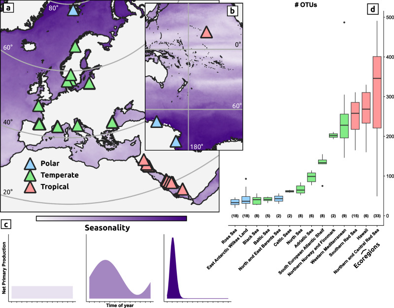
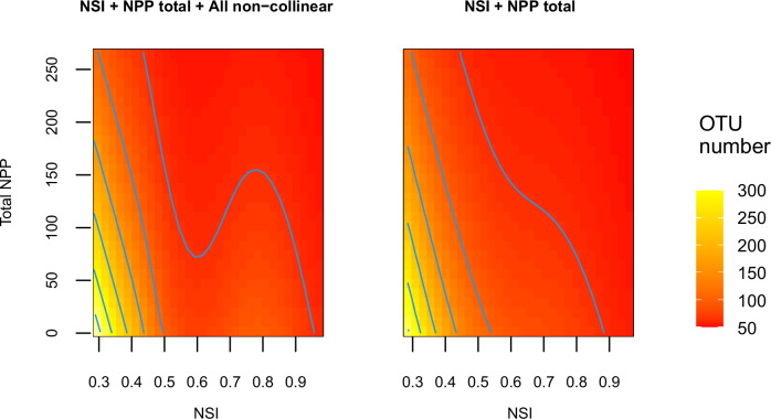
A pattern of increasing species richness from the poles to the equator is frequently observed in many animal taxa. Ecological limits, determined by the abiotic conditions and biotic interactions within an environment, are one of the major factors influencing the geographical distribution of species diversity. Energy availability is often considered a crucial limiting factor, with temperature and productivity serving as empirical measures. However, these measures may not fully explain the observed species richness, particularly in marine ecosystems. Here, through a global comparative approach and standardised methodologies, such as Autonomous Reef Monitoring Structures (ARMS) and DNA metabarcoding, we show that the seasonality of primary production explains sessile animal richness comparatively or better than surface temperature or primary productivity alone. A Hierarchical Generalised Additive Model (HGAM) is validated, after a model selection procedure, and the prediction error is compared, following a cross-validation approach, with HGAMs including environmental variables commonly used to explain animal richness. Moreover, the linear effect of production magnitude on species richness becomes apparent only when considered jointly with seasonality, and, by identifying world coastal areas characterized by extreme values of both, we postulate that this effect may result in a positive relationship in environments with lower seasonality.

Fig. 1. Deployment locations and richness of the ARMS investigated in this study.

a Deployment locations for the Autonomous Reef Monitoring Structures (ARMS) investigated by Carvalho et al. and Pearman et al., as well as data obtained from the ARMS–Marine Biodiversity Observation Network (ARMS-MBON) programme. b Deployment locations for the ARMS investigated by Nichols et al. as well as the ones from Antarctica. Purple tone shows the degree of seasonality, as described in box (c). c Schematic representation of the dynamics of Net Primary Production at different seasonality levels, following the same representation used in Berger and Wefer. Lighter purple tones reflect a condition where primary production is constant throughout the year, whereas darker tones indicate higher seasonality, with most of the yearly production mostly occurring in a specific season. d Tukey-style boxplots showing the distribution of the number of molecular Operational Taxonomic Units (mOTUs) for the structures in each ecoregion investigated. The sample number onto which boxplots are calculated is shown in brackets above the x axis labels, and refers to technical replicates. The lower and upper hinges correspond to the 25th and 75th percentiles, while the central line refers to the median. The upper whisker extends to the largest value no further than 1.5 * inter-quantile range (IQR) from the 75th percentile, while the lower extends to the smallest value at most 1.5 * IQR of the 25th percentile. All data points outside these ranges are plotted individually. These boxplots are shown only for the purpose of indicating the variability of mOTU richness across all the ecoregions. The triangles’ and boxplots colours refer to the latitudinal zone in which the deployment took place, and the boxplots are ordered by the median of the number of mOTUs of the samples for each ecoregion. Ecoregions and latitudinal zones were defined following Spalding et al.. The map was created using QGIS (version 3.14), the coastline contour was downloaded from the Global Self-consistent, Hierarchical, High-resolution Geography database (GSHHG, version 2.3.7).

Fig. 2. Contour plots of HGAM models predictions.

The predictions of the number of mOTUs corresponding to the smoothers of total NPP and NSI in the HGAM models obtained. Yellow tiles indicate higher mOTUs number, red tiles lower. The total NPP and NSI values are on the y and x axis respectively. The blue lines correspond to contour values of OTU number prediction, increasing by a factor of 50, as reported in the colour bar of the figure.

Fig. 3. Partial effect plots of alternative HGAM models.

Smoothers of the models fitted with single variables usually used in describing benthic metazoan richness (Sea Surface Temperatures, Chlorophyll and Net Primary Productivity means and total), in addition to the NSI. The component smooth function is plotted on the scale of the linear predictor in the y-axis. The table reports the χ² and p values (two-sided chi-square test) of each single model.

Fig. 4. Violin plots of prediction errors.

Violin plots showing the root-mean-square error (RMSE) values obtained in the cross-validation process for different HGAM models. Each violin refers to the RMSE values obtained for all 100 random validation datasets of a single model and has been ordered according to the median of all RMSE values. Tukey-style boxplots inside the violin plots show the 25th and 75th percentiles, as lower and upper hinges respectively, while the central line refers to the median. The upper whisker extends to the largest value no further than 1.5 * inter-quantile range (IQR) from the 75th percentile, while the lower extends to the smallest value at most 1.5 * IQR of the 25th percentile. All data points outside these ranges are plotted individually.

Fig. 5. Smoother linearity of total NPP in HGAM models.

Predictions effect (smoothers) for the models including the total NPP and tested on the validation datasets in the cross-validation process. a The prediction effects of the model including total NPP on the number of mOTUs. Dashed, black lines show the smoothing obtained using the command ‘geom_smooth’ in ggplot and the arguments ‘method = gam’ ‘formula = y ~ s(x)’ on the upper and lower confidence intervals of each smoother in the validation datasets. b The prediction effect of the model including total NPP and NSI on the validation datasets with fixed values of the NSI at different levels of seasonality (from 0.4 to 0.8). Solid, stroked lines are produced using the command ‘geom_smooth’ in ggplot and adopting the arguments ‘method = gam’ and ‘formula = y ~ s(x)’. The unit for total NPP is reported in the ‘Methods’ section.

Fig. 6. Graphic representation of the percentage of random point falling on coastal areas with high energy availability in each ecoregion.

a 5% extrapolation areas for the mOTU richness prediction of the smoothers in the model including NSI and total NPP. b Density plot of all random points generated in the 0.04 degrees coastal areas of the Global Self-consistent, Hierarchical, High-resolution Geography database (GSHHG) world coastlines plotted with the corresponding total NPP ( y axis) and NSI (x axis) values from the global rasters of those variables. Each tile can include a minimum of 1 point. Red shaded area represents the high energy availability combinations of total NPP and NSI values (NSI < 0.4 and total NPP > 75 g m⁻² year⁻¹), and matches the low confidence area of the prediction in box (a). c Ecoregions are coloured based on the percentage of number of points falling on high energy availability coastal areas in respect to the total number of random points. d As per box (c), but based on the percentage of points falling on low seasonality areas (NSI < 0.4), irrespective of total NPP values.

References

1. Fine, P. V. A. Ecological and evolutionary drivers of geographic variation in species diversity. Annu. Rev. Ecol. Evol. Syst.46, 369–392 (2015).
1. Pontarp, M. et al. The latitudinal diversity gradient: novel understanding through mechanistic eco-evolutionary models. Trends Ecol. Evol.34, 211–223 (2019). - PubMed
1. Chaudhary, C., Saeedi, H. & Costello, M. J. Marine species richness is bimodal with latitude: a reply to Fernandez and Marques. Trends Ecol. Evol.32, 234–237 (2017). - PubMed
1. Fernandez, M. O. & Marques, A. C. Diversity of diversities: a response to Chaudhary, Saeedi, and Costello. Trends Ecol. Evol.32, 232–234 (2017). - PubMed
1. Gili, J.-M., Coma, R., Orejas, C., López-González, P. J. & Zabala, M. Are Antarctic suspension-feeding communities different from those elsewhere in the world? Polar Biol.24, 473–485 (2001).