Proteome-wide copy-number estimation from transcriptomics

Abstract

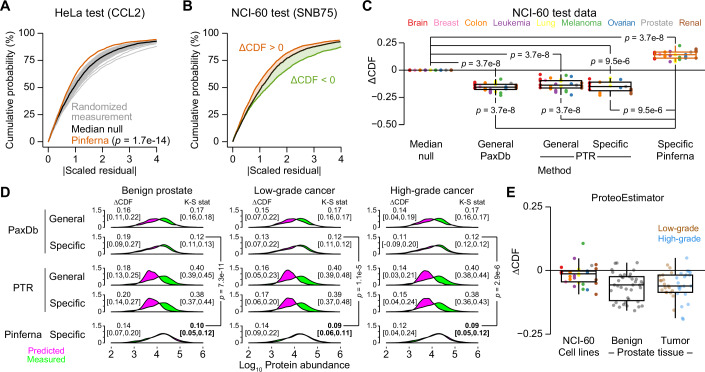
Protein copy numbers constrain systems-level properties of regulatory networks, but proportional proteomic data remain scarce compared to RNA-seq. We related mRNA to protein statistically using best-available data from quantitative proteomics and transcriptomics for 4366 genes in 369 cell lines. The approach starts with a protein's median copy number and hierarchically appends mRNA-protein and mRNA-mRNA dependencies to define an optimal gene-specific model linking mRNAs to protein. For dozens of cell lines and primary samples, these protein inferences from mRNA outmatch stringent null models, a count-based protein-abundance repository, empirical mRNA-to-protein ratios, and a proteogenomic DREAM challenge winner. The optimal mRNA-to-protein relationships capture biological processes along with hundreds of known protein-protein complexes, suggesting mechanistic relationships. We use the method to identify a viral-receptor abundance threshold for coxsackievirus B3 susceptibility from 1489 systems-biology infection models parameterized by protein inference. When applied to 796 RNA-seq profiles of breast cancer, inferred copy-number estimates collectively re-classify 26-29% of luminal tumors. By adopting a gene-centered perspective of mRNA-protein covariation across different biological contexts, we achieve accuracies comparable to the technical reproducibility of contemporary proteomics.

Keywords: CCLE; CVB3; Pinferna; SWATH; TMT.

Figure 1. Meta-assembly and inference of conditional mRNA-to-protein relationships for 4366 human genes.

(A) Data fusion and model discrimination. (1) Tandem mass tag (TMT) proteomics of 375 cancer cell lines (Nusinow et al, 2020) were calibrated to a proportional scale based on sequential window acquisition of all theoretical mass spectra (SWATH) proteomics of CAL51 and U2OS cells (PXD003278; PXD000954). (2) SWATH-scaled proteins were regressed using three models that incorporate transcript abundance from RNA sequencing (RNA-seq) to different extents: median (M), no contribution of mRNA; hyperbolic-to-linear (HL) relationship incorporating mRNA of the gene, $a\bullet \left(\frac{b\bullet mRNA}{c+mRNA}+mRNA\right)$; HL + least absolute shrinkage and selection operator (LASSO) regressors with mRNAs other than the gene of interest. (3) Model selection for each gene was based on the Bayesian Information Criterion. The number of genes selected in each class is indicated. (4) New samples profiled by RNA-seq were used with the calibrated models to make protein inference from RNA (Pinferna) predictions. The number of proteins measured per sample or number of samples with data per protein is shown at each step as the median with the range in brackets. (B) Reliable cross-calibration of the TMT and SWATH meta-assembly. Step 1 of (A) was performed with CAL51 data alone and the SWATH-scaled TMT proteomics of U2OS cells compared with data obtained directly by SWATH. The reciprocal cross-calibration is shown in Fig. EV1B. (C–E) Representative M, HL, and HL + LASSO genes. Proportional protein copies per cell were regressed against the mRNA abundance normalized as transcripts per million (TPM). Evidence for model selection is shown in Fig. EV1C–E. Data information: For (B), Pearson’s R and Spearman’s ρ are shown. For (C–E), best-fit calibrations ± 95% confidence intervals are overlaid on the proteomic–transcriptomic data from n = 369 cancer cell lines.

Figure 2. Pinferna model selection is consistent with known biological mechanisms and mRNA-to-protein relationships.

(A) Gene ontology (GO) enrichments for M genes. The largest non-redundant GO term is shown with the fold enrichment (FE) and false discovery rate-corrected p value (q). The complete list of GO enrichments for each relationship class is available in Dataset EV5. (B) HL outperforms competing mRNA-to-protein relationships. Models encoding linear, hyperbolic, three-parameter logistic, and HL relationships were built for all genes and compared by Bayesian Information Criterion (BIC). Results are shown as the smoothed density of BIC differences (∆BIC) relative to the best model for that gene (∆BIC = 0). Distributions of BIC weights (Wagenmakers and Farrell, 2004) are shown in Fig. EV2D. (C, D) HL captures different empirical classes of mRNA-to-protein relationships. Log-concave genes (C) saturate at high mRNA abundance, whereas log-convex genes (D) plateau at low mRNA abundance. The remaining genes exhibited characteristics of both fits or linear relationships to varying degrees (Fig. EV2G–I). (E, F) Ratio compression of a log-convex gene. The indicated cell lines were immunoblotted for SERPINB6 along with vinculin and tubulin as loading controls (E), and loading-normalized SERPINB6 abundance was quantified relative to the median copy number for these cell lines in the meta-assembly. Observations were compared to the meta-assembly (F) assuming direct proportionality (blue). (G) Feature weights of HL + LASSO genes are biologically sensible. Smoothed densities of LASSO feature weights (indicating strength and direction of modulation for an HL fit) among mRNAs encoding subunits of the proteasome (blue) and the ribosome (red) are shown. (H) HL + LASSO features are highly enriched for STRING interactions. For each HL + LASSO gene, LASSO-selected features were replaced with random genes to build a null distribution for finding binary interactions in STRING (Szklarczyk et al, 2023). The actual number of STRING interactions among HL + LASSO genes of Pinferna is indicated. Data information: For (B), n = 4366 genes. For (F), n = 3 biological replicates. For (G), n = 127 feature weights (blue) or 397 feature weights (red). For (H), n = 10,000 randomizations.

Figure 3. Pinferna outperforms randomized measurements and competing methods for proportional protein abundance estimation.

(A) Pinferna compared to random protein-specific measurements. Model predictions were nondimensionalized as a scaled residual by subtracting the measured abundance, dividing by the standard deviation of the SWATH-scaled protein measured across the meta-assembly, and taking the absolute value (|Scaled residual | ). The |Scaled residual| cumulative density was compared to randomized measurements drawn from the SWATH-scaled proteomic data for each gene. Randomized measurements were iterated 100 times (gray) to identify a median null (black) that served as a null distribution for model assessment. Left-shifted distributions indicate improved proteome-wide accuracy (relative to each protein’s variability) compared to protein-specific randomized measurements. (B) Aggregate performance assessment of protein abundance predictions. The difference in cumulative density functions between test predictions and the median null distribution (∆CDF) was integrated to identify approaches that performed better (∆CDF > 0, orange) or worse (∆CDF < 0, green) than protein-specific randomized measurements. Data are from a prediction of Pinferna (orange) and tissue-specific protein-to-mRNA ratio (PTR; green). (C) Pinferna is superior to empirical guessing in cultured cell lines. ∆CDF values were calculated for NCI-60 cell lines (PRJNA433861; (Guo et al, 2019)) excluded from model training (Fig. 1A) and organized by cancer type. PaxDb (Wang et al, 2015) and PTR (Eraslan et al, 2019) were used generically or in a tissue-specific way as alternative approaches for proportional quantification (“Methods”). A cell line-specific PaxDb estimate was only available for U251 cells. (D) Pinferna reconstitutes proteome-wide distributions of proportional copy numbers in normal prostate tissue (left; case L1N), low-grade prostate cancer (middle; case M7U), and high-grade prostate cancer (right; case H9T) (PRJNA579899; PXD004589; Dataset EV6). (E) ProteoEstimator, the best-performing model of the NCI–CPTAC DREAM proteogenomic challenge (Yang et al, 2020), does not accurately predict protein copy numbers when mapped to a proportional scale (“Methods”). Data information: For (A), Pinferna predictions of HeLa cells (orange; PRJNA437150; PXD009273) were compared to the null distribution by K-S test. For (C, E), n = 5 brain, 1 breast, 3 colon, 4 leukemia, 4 lung, 3 melanoma, 3 ovarian, 1 prostate, 5 renal cell lines. For (D, E), n = 39 normal prostate samples, 19 low-grade, 21 high-grade prostate cancers. For (D), the median ∆CDF and K-S statistic (K-S stat) are reported with range in brackets. For (C, D), differences between groups were assessed by paired sign-rank tests with Šidák correction. Box-and-whisker plots show the median (horizontal line), interquartile range (IQR, box), and an additional 1.5 IQR extension (whiskers) of the data.

Figure 4. Simulating degrees of human cardio-susceptibility to coxsackievirus B3 (CVB3) infection based on inferred abundance differences in CVB3 receptors.

(A) An in silico model of CVB3 initiated by its receptors CD55 and CXADR. After binding, the virus undergoes internalization, replication, and escape. The viral life cycle is mathematically modeled with 54 ordinary differential equations (ODEs; MODEL2110250001). (B) Distribution of viral load over time from 1489 human heart samples. Inferred abundances of CD55 and CXADR from each sample were used to simulate CVB3 infection. Each model run consisted of 100 simulated infections up to 24 h with a coefficient of variation in model parameters of 5%. Viral loads (gray) at the indicated time points are shown along with the estimated point of lysis. (C) Four modes of infection susceptibility to terminal CVB3 infection. Viral load at 24 h was replotted from (B) fit to a Gaussian mixture model (black) of three components (purple, green, yellow). Relative population densities in each of the susceptibility groups is shown along with the estimated point of lysis. (D, E) Distribution of mRNA abundances for CD55 (D) and CXADR (E) normalized as TPM. (F, G) Distribution of inferred protein copy numbers per cell for CD55 (F) and CXADR (G) with each sample colored by its susceptibility. (H–K) AC16 cardiomyocytes were stably transduced with doxycycline (DOX)-inducible CXADR-V5 (iCAR), induced for 30 min (H, I) or 60 min (J, K) and immunoblotted for CXADR with vinculin and GRB2 as loading controls (H, J) or infected with CVB3 (multiplicity of infection = 5) for 6 h and quantified for VP1 (I, K). Immunoblots of (H, J) are quantified in Fig. EV4I,K, and representative immunoblots of (I, K) are shown in Fig. EV4J,L. The average CXADR copy number per cell is indicated for each group (I, K). Data information: For (B, C), the black diamond indicates the mean estimated lytic yield ± s.d. (Dunnebacke and Reaume, ; Griffiths et al, ; Lopacinski et al, 2021). For (B–G), n = 1489 heart samples. For (I, K), box-and-whisker plots show the median VP1 (horizontal line), mean VP1 (asterisk), interquartile range (IQR, box), and an additional 1.5 IQR extension (whiskers) from n = 4 biological replicates. Differences were assessed with a one-way ANOVA followed by Tukey’s Honest Significant Difference post hoc test for DOX- and iCAR-associated increases. n.d. no difference.

Figure 5. Inferred proteomics reassigns luminal A/B transcriptomic subtypes of breast cancer.

(A) Reorganization of five consensus clusters defined by RNA-seq (left) and Pinferna (right) for breast cancers in The Cancer Genome Atlas (Ciriello et al, 2015). Clusters were determined by Monte Carlo consensus clustering (John et al, 2020) and colored according to the dominant PAM50 subtype of each cluster. Samples that did not change clusters are transparent in the background while samples that changed are opaque in the foreground. Lum A: Luminal A; Lum B: Luminal B. (B) Reassigned samples are predominated by luminal A/B PAM50 subtypes. (Left) Proportion of each subtype among samples that were reassigned. (Right) Percent reassignments for each subtype. The average overall reassignment rate is shown as a null reference (186/796 = 23%; gray dashed) with the 90% hypergeometric confidence interval (black) for each subtype. BL is Basal-like, H2 is HER2 + , LA is Luminal A, LB is Luminal B, and NL is Normal-like. (C–F) Cluster-reorganizing genes are highly dependent on other genes. (Left) Concordance between SWATH-scaled measurements and the HL fit ± LASSO in the meta-assembly. Perfect concordance is given by the red dashed line. Pink points in (E) are samples with TPM = 0 for CTNNA2. (Right) STRING interactions (edges) among the target gene (orange) and its LASSO-selected features (black). Edge thickness (gray) reflects the confidence of the interaction as determined by STRING. Thicker lines represent a higher confidence score. Line lengths are arbitrary. Data information: For (A), n = 796 breast cancers. For (B), reassignment enrichments were determined by hypergeometric test, *P = 2.2e-4 (BL), 1.9e-2 (H2), 4.1e-2 (LA), and 3.1e-2 (LB). For (C–F), n = 369 cell lines.

Figure 6. LASSO features of CDK4 include causal dependencies.

(A, B) Knockdown of NUP37 increases CDK4 abundance in B2B1 breast epithelial cells (Wang et al, 2023). (C, D) Overexpression of inducible NUP37 (iNUP37) decreases CDK4 abundance in B2B1 breast epithelial cells. (E, F) Overexpression of iNUP37 decreases CDK4 abundance in MCF7 luminal breast cancer cells. (G, H) Residual DNM1L protein after knockdown correlates with CDK4 abundance in T47D (G) and ZR751 (H) luminal breast cancer cells. Actin was used as a housekeeping control not used for loading normalization (“Methods”). Quantities are scaled to shScramble control samples. Data information: For (A, C, E), representative immunoblots for NUP37 and CDK4 are shown with vinculin and tubulin (A, C) or p38 (E) as loading controls and FLAG (C, E) to confirm ectopic expression of iNUP37 or luciferase (luc) control. For (B, D, F), immunoblot results are summarized as the mean total NUP37 (endogenous (B, D, F) and induced (D, F)) or CDK4 ± s.e.m. of n = 6 biological replicates. Differences were assessed by one-sided t test. For (G, H), representative immunoblots for DNM1L and CDK4 are shown with vinculin and p38 as loading controls and actin as a housekeeping control. Data are summaries from n = 6 biological replicates.

Figure EV1. Calibration for the proteomic meta-assembly and model selection examples.

(A) SWATH–TMT scaling factor estimation and calibration of the proteomic meta-assembly. Scaling factors were estimated for each protein by dividing the SWATH intensity by the TMT intensity in U2OS and CAL51 when both data types were available and averaging (avg) the two ratios when possible. The gene-specific scaling factors were used to convert the entire TMT dataset (bold) to proportional protein abundances. (B) The reciprocal cross-calibration to that shown in Fig. 1B. Step 1 of Fig. 1A was performed with U2OS data alone and the SWATH-scaled TMT proteomics of CAL51 cells compared with data obtained directly by SWATH. (C–E) Model selection of the representative genes shown in Fig. 1C–E. Proportional protein copies per cell were regressed against the mRNA abundance normalized as transcripts per million (TPM). Data are fit with M, HL, and HL + LASSO models. The BIC was used to discriminate the best model for each fit, and BIC weights (w) are shown in parentheses to indicate the relative best-model probability. The lowest BIC is indicated. (F) BIC weights (BICw) for each model fit to M, HL, or HL + LASSO ( + LASSO) genes. Range of weights for genes with model ambiguity (two models with a BICw ≥0.4) are boxed (gray) with the percentage indicated. Data information: For (B), Pearson’s R and Spearman’s ρ are shown. For (C–E), n = 369 cancer cell lines. For (F), box-and-whisker plots show the median BICw (horizontal line), interquartile range (IQR, box), and an additional 1.5 IQR extension from the box edge (whiskers) from n = 4366 genes.

Figure EV2. Extended characterization of M and HL mRNA-to-protein relationship classes.

(A, B) M genes do not exhibit longer half-lives compared to other relationship classes. Half-lives for proteins were obtained from (Zecha et al, 2018) and plotted by frequency (A) or as an empirical cumulative distribution function (B) for all genes (gray) and M genes (green). (C) M genes are more abundant by mRNA compared to other relationship classes. mRNA abundance was normalized as TPM and placed on a log scale with a pseudocount of 1. Cumulative distribution functions are shown for M genes (green), HL genes (purple), and HL + LASSO genes (orange). (D) Distribution of BIC weights (BICw) for models encoding linear, hyperbolic, three-parameter logistic, and HL relationships shown in Fig. 2B. (E, F) Log-convex patterns arise when mRNA and protein abundances recover from transient perturbations to steady-state values. A simple transcription–translation model (E) was reduced by 50% and randomly sampled at 10 time points (red) during the return to steady state (s.s.). For the model, the following dimensionless rate parameters were used: k_txn = 1; k_trl = 1; k_{RNA_deg} = 0.1; k_{protein_deg} = 0.01. The model was simulated 100 times with lognormally distributed parameter noise (coefficient of variation = 10%) and the joint observation of mRNA and protein abundances (n = 10 time points x 100 simulations) is shown in (F). (G–I) Examples of other HL relationships besides those of Fig. 2C, D: mixed concavity (G), weakly linear (H), and strongly linear (I) relationships. Data information: For (A, B), n = 7029 genes (gray) and 334 genes (green). For (C), n = 395 genes (green), 2569 genes (purple), and 1402 genes (orange). Distributions were compared by K-S test with Šidák correction for multiple-hypothesis testing. For (D), n = 4366 genes.

Figure EV3. Robustness of Pinferna predictions.

(A, B) Cumulative distribution of scaled residuals degrades with decreasing correlation (A) and slope (B) between predicted and measured values. A synthetic dataset was created by taking the median TPM and protein value for each gene among 12 HeLa cell lines (Liu et al, 2019) and using perturbations of the synthetic data as a prediction. The median null for this dataset relative to Pinferna is shown for reference. To disrupt correlations (A), Gaussian white noise with increasing variance was added to the measured HeLa protein abundances to achieve the indicated Pearson correlations. Measured protein abundances were separately multiplied by the indicated slope while retaining a linear relationship (B). (C, D) Prediction accuracy is not dependent on SWATH analytical details. Cumulative distribution plots comparing Pinferna and median-null predictions for paired RNA-seq–SWATH datasets of 12 HeLa derivatives (PRJNA437150; PXD009273) named as in the publication (Liu et al, 2019). Proteins were re-quantified from raw SWATH data processed exactly like the meta-assembly (“Methods”) (C); or, protein quantities were taken directly from the publication (Liu et al, 2019) (D). Results from the re-quantified CCL2 L2 derivative are reprinted from Fig. 3A. (E) Prediction accuracy is not heavily dependent on RNA-seq read depth. Count-based RNA-seq data for the HeLa lines was averaged and iteratively downsampled (gray) and TPM values re-estimated before making proteome-wide copy-number predictions with Pinferna. See Fig. 3B for an explanation of ∆CDF. (F) Prediction accuracy is not dependent on RNA-seq analytical details. Pinferna predictions were made using TPM values taken directly from the original publication (Reinhold et al, 2019), and ∆CDF values were calculated for NCI-60 cell lines excluded from model training (Fig. 1A) and organized by cancer type. Data information: For (E), n = 100 iterations. For (F), n = 5 brain, 1 breast, 3 colon, 4 leukemia, 4 lung, 3 melanoma, 3 ovarian, 1 prostate, 5 renal cell lines. Differences between groups were assessed by paired sign-rank tests with Šidák correction. For (E, F), box-and-whisker plots show the median ∆CDF (horizontal line), interquartile range (IQR; box), and an additional 1.5 IQR extension (whiskers) of the data.

Figure EV4. Calibrated protein inferences of CD55 and CXADR yield disease-related predictions of coxsackievirus B3 (CVB3) susceptibility.

(A) Distribution of CD55 abundance (Dataset EV7) separated by source data: EGA (brown; EGAS00001002454), GTEx (gray; phs000424.v9.p2), MAGNet (blue; GSE141910). (B) CXADR is upregulated in failing hearts. CXADR abundance (Dataset EV7) was stratified by heart health and colored by source data as in (A). (C, D) Calibration plots (orange (C); purple (D)) and Pinferna predictions for CD55 (C) and CXADR (D) in human heart samples (Heart RNA-seq; red). CD55 deviations from the smoothed best fit are caused by cardiac-specific features in the HL + LASSO regressions. (E, F) CD55–CXADR coregulation is increased at the protein level (F) compared to the mRNA level (E). (G) Replotted histogram of Fig. 4C separated by heart health (Dataset EV7). (H) Predicted prevalence of susceptibility groups based on randomized measurements. After linearly scaling to randomized abundances of CD55 and CXADR, CVB3 infections were simulated for 1489 heart samples as in Fig. 4B. The 24-h end states were quantified by the percentage of samples with resistant ([CVB3 virions] = 0 nM), sublytic (0 nM < [CVB3 virions] < 36 nM), and lytic ([CVB3 virions] ≥ 36 nM) phenotypes (Fig. 4C). Pinferna-derived percentages are overlaid in red. Results from the randomized simulations are connected, and densities in each group are shown by a violin plot in the background. (I–L) AC16 cardiomyocytes were stably transduced with doxycycline (DOX)-inducible CXADR-V5 (iCAR), induced for 30 min (I, J) or 60 min (K, L) and quantified for CXADR (I, K) or infected with CVB3 (multiplicity of infection = 5) for 6 h and immunoblotted for VP1 with vinculin and GRB2 as loading controls (J, L). Representative immunoblots of (I, K) are shown in Fig. 4H, J, and immunoblots of (J, L) are quantified in Fig. 4I, K. Data information: For (B–F), n = 1489 heart samples. For (B), differences between groups were assessed by rank-sum test. For (C, D), best-fit calibrations ± 95% confidence intervals are overlaid on the proteomic–transcriptomic data from n = 369 cancer cell lines. For (E, F), the Pearson R is shown with 95% confidence interval in brackets calculated by the Fisher Z transformation. For (H), n = 100 randomizations. For (I, K), n = 4 biological replicates calibrated against a five-point standard curve of AC16-CAR cells fit as a linear model.

References

1. Agren R, Bordel S, Mardinoglu A, Pornputtapong N, Nookaew I, Nielsen J (2012) Reconstruction of genome-scale active metabolic networks for 69 human cell types and 16 cancer types using INIT. PLoS Comput Biol 8:e1002518 - PMC - PubMed
1. Ahrne E, Molzahn L, Glatter T, Schmidt A (2013) Critical assessment of proteome-wide label-free absolute abundance estimation strategies. Proteomics 13:2567–2578 - PubMed
1. Alvarez MJ, Shen Y, Giorgi FM, Lachmann A, Ding BB, Ye BH, Califano A (2016) Functional characterization of somatic mutations in cancer using network-based inference of protein activity. Nat Genet 48:838–847 - PMC - PubMed
1. Bajikar SS, Wang CC, Borten MA, Pereira EJ, Atkins KA, Janes KA (2017) Tumor-suppressor inactivation of GDF11 occurs by precursor sequestration in triple-negative breast cancer. Dev Cell 43:418–435 e413 - PMC - PubMed
1. Barrett T, Wilhite SE, Ledoux P, Evangelista C, Kim IF, Tomashevsky M, Marshall KA, Phillippy KH, Sherman PM, Holko M et al (2013) NCBI GEO: archive for functional genomics data sets-update. Nucleic Acids Res 41:D991–D995 - PMC - PubMed
LinkOut - more resources