Thin Conducting Films: Preparation Methods, Optical and Electrical Properties, and Emerging Trends, Challenges, and Opportunities

Abstract

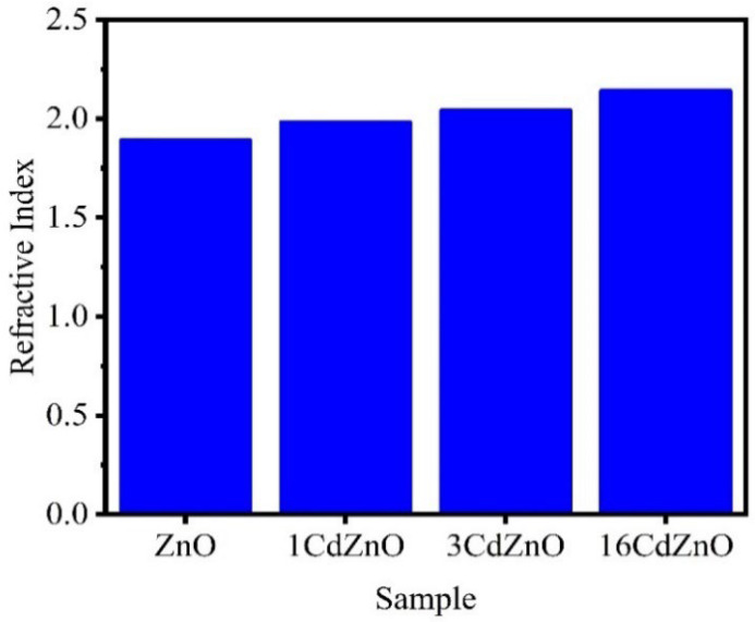
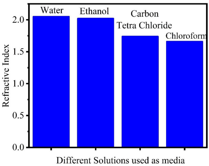
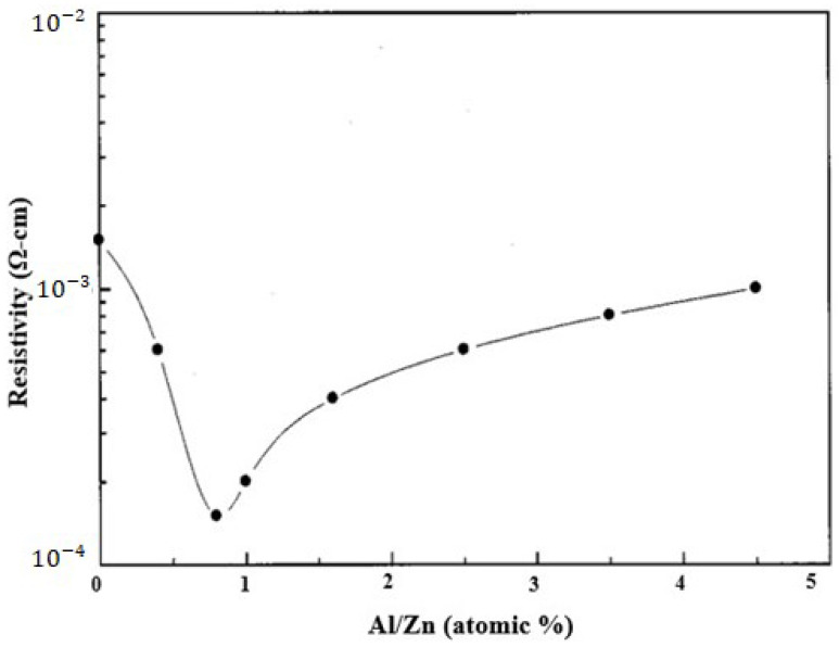
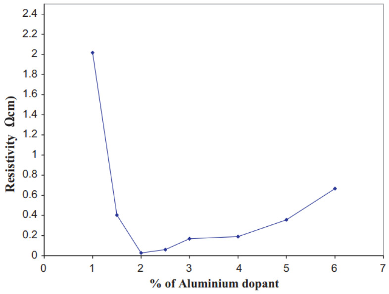
Thin conducting films are distinct from bulk materials and have become prevalent over the past decades as they possess unique physical, electrical, optical, and mechanical characteristics. Comprehending these essential properties for developing novel materials with tailored features for various applications is very important. Research on these conductive thin films provides us insights into the fundamental principles, behavior at different dimensions, interface phenomena, etc. This study comprehensively analyzes the intricacies of numerous commonly used thin conducting films, covering from the fundamentals to their advanced preparation methods. Moreover, the article discusses the impact of different parameters on those thin conducting films' electronic and optical properties. Finally, the recent future trends along with challenges are also highlighted to address the direction the field is heading towards. It is imperative to review the study to gain insight into the future development and advancing materials science, thus extending innovation and addressing vital challenges in diverse technological domains.

Keywords: electrical properties; future trends in TCFs; optical properties; preparation/methodology; thin conducting film (TCF); thin film.

Figure 1

Different types of PVD techniques for depositing TCFs.

Figure 2

The thermal evaporation phenomenon.

Figure 3

EBE technique.

Figure 4

MBE technique.

Figure 5

Schematic representation of laser ablation.

Figure 6

Resistance heating evaporation technique.

Figure 7

Ion plating deposition technique.

Figure 8

Physical sputtering’s energy regimes. Reproduced from [98] under permissions from copyright clearance center.

Figure 9

RF sputtering system’s working chamber.

Figure 10

Reactive sputtering technique. Reproduced from [111] under permissions from copyright clearance center.

Figure 11

Setup for IBS deposition. Reproduced from [114] under permissions from copyright clearance center.

Figure 12

(a) Diode sputtering; (b) triode sputtering.

Figure 13

Magnetron sputtering technique.

Figure 14

LPCVD system for ZnO nanowires.

Figure 15

PECVD process.

Figure 16

PLD process.

Figure 17

Schematic representation of APCVD technique.

Figure 18

An illustration of the CBD process.

Figure 19

Spin-coating deposition technique.

Figure 20

Schematic for the direct electrodeposition of conductive polymer onto a magnesium working electrode in an electrochemical cell.

Figure 21

Overview showcasing two instances of sol–gel synthesis: (a) colloidal sol films and (b) colloidal sol powder that has been gelled.

Figure 22

Schematic of a spray pyrolysis deposition system.

Figure 23

Diagrammatic representation of the following steps: (a–c) the setup for the anodization process and the deposition of the aluminum film; (d–f) Al film at various anodization stages (the cross-sectional view); and (g) the creation of the PDLC-based smart window device using anodized nanoporous aluminum (AAO/Al). The PDLC smart window can be in one of two states: (h) opaque or OFF or (i) transparent or ON. Reproduced from [180] under permissions from copyright clearance center.

Figure 24

An illustration of the vertical MOCVD reactor.

Figure 25

Spectra of absorption of forms of PANI: (a) leucoemeraldine base; (b) emeraldine. Reproduced from [304] under permissions from copyright clearance center.

Figure 26

Different light-emitting polymers studied by Gioti et al. [310]: (a) ${\epsilon }_1\left(\omega \right)$; (b) ${\epsilon }_2\left(\omega \right)$. Reproduced from [310] under permissions from copyright clearance center.

Figure 27

Effects on the square of the absorption coefficient for different Al dopant concentrations with changing photon energy. Reproduced from [214] under permissions from copyright clearance center.

Figure 28

Variations in $({\alpha h\vartheta )}^2$ and incident photon energy for thin films created with varying aluminum doping concentrations. Reproduced from [216] under permissions from copyright clearance center.

Figure 29

Absorption spectra of CuI at different substrate temperatures. Reproduced from [190] under permissions from copyright clearance center.

Figure 30

Absorption coefficient vs wavelength. Reproduced from [335] under permissions from copyright clearance center.

Figure 31

Optical transmittance of glass and AZO films placed on glass at (a) uncoated, (b) 400 °C, and (c) 500 °C with different annealing temperatures. Reproduced from [214] under permissions from copyright clearance center.

Figure 32

The transmittance spectra of films created at various initial aluminum atomic ratios. Reduced [216] under permissions from copyright clearance center.

Figure 33

ITO film optical transmittance spectra with varying Sn doping concentrations. Reproduced from [202] under permissions from copyright clearance center.

Figure 34

Grain size fluctuation with varying amounts of Sn doping. Reproduced from [202] under permissions from copyright clearance center.

Figure 35

Shows the evolution of the ITO films’ (a) thickness and (b) transmittance at varied powers and deposition times. Reproduced from [325] under permissions from copyright clearance center.

Figure 36

ITO films’ transmittance after being deposited at varied powers and deposition durations: (a) 20 min; (b) 40 min; (c) 60 min. Reproduced from [325] under permissions from copyright clearance center.

Figure 37

Changes in the transmittance with different deposition techniques reported by other authors.

Figure 38

Transmittance spectra of CuI thin films deposited at various substrate temperatures. Reproduced from [359] under permissions from copyright clearance center.

Figure 39

CuI thin-film transmission spectra at various annealing temperatures. The absorption spectra of CuI thin films are displayed in the inset. Reproduced from [54] under permissions from copyright clearance center.

Figure 40

CuI film transmissivity spectra at (a) 1 at. %, 2 at. %, and 3 at. %; (b) undoped, 4 at. %, and 5 at. %. Reproduced from [191] under permissions from copyright clearance center.

Figure 41

Variations in transmittance with wavelength for INO. Reproduced from [372] under permissions from copyright clearance center.

Figure 42

Changes in the transmittance with changes in the substrate temperature for INO. Reproduced from [342] under permissions from copyright clearance center.

Figure 43

Effects of temperature on the transmittance for INO. Reproduced from [344] under permissions from copyright clearance center.

Figure 44

Changes in (a) transmittance and (b) reflectance with the increasing doping concentration of vanadium. Reproduced from [374] under permissions from copyright clearance center.

Figure 45

Variations in transmittance with changing oxygen pressure. Reproduced from [342] under permissions from copyright clearance center.

Figure 46

Variations in transmittance with annealing temperature. Reproduced (a) from [333]; (b) from [334] under permissions from copyright clearance center.

Figure 47

Changes in the transmittance with increasing (a) Al dopant [377] and (b) Mn dopant [378] in CdO thin films. Reproduced from [377,378] under permissions from copyright clearance center.

Figure 48

Influence of (a) Al dopant [335] and (b) La dopant [380] on the transmittance of CdO thin films. Reproduced from [335,380] under permissions from copyright clearance center.

Figure 49

The relationship between reflectance and substrate temperature for ZnO: Al films formed at 150–370 °C. Reproduced from [221] under permissions from copyright clearance center.

Figure 50

Variations in CdO’s reflectance with the doping concertation of Al. Reproduced from [339] under permissions from copyright clearance center.

Figure 51

Changes in the reflectance with substrate temperature. Reproduced from [342] under permissions from copyright clearance center.

Figure 52

Variations in refractive index with film thickness.

Figure 53

Refractive index vs. film thickness plotted from the data provided by Reddy et al. [223].

Figure 54

Changes in the refractive index with the changing SnO₂ content.

Figure 55

ITO films produced at different temperatures and their refractive indices.

Figure 56

Variations in the refractive index with doping concentrations. Reproduced from [339] under permissions from copyright clearance center.

Figure 57

Changes in the refractive index for CdO doping in ZnO thin films.

Figure 58

Variations in the refractive index when using different solution media. The column graph is plotted using the data available from Kariper’s investigation.

Figure 59

The correlation between AZO thin films’ resistance and aluminum dopant concentration in the solution. Reproduced from [214] under permissions from copyright clearance center.

Figure 60

Resistivity for ZnO: Al films with increasing aluminum doping concentration. Reproduced from [216] under permissions from copyright clearance center.

Figure 61

The relationship between the annealing temperature and the resistivity of AZO thin films. Reproduced from [214] under permissions from copyright clearance center.

Figure 62

Resistivity of ZnO: Al films for different deposition techniques.

Figure 63

CuI thin films’ resistivity and figure of merit as a function of annealing temperature. Reproduced from [54] under permissions from copyright clearance center.

Figure 64

Variations in CuI film resistivity at varying iodine doping concentrations. Reproduced from [191] under permissions from copyright clearance center.

Figure 65

Changes in the electrical resistivity with increasing temperature. Reproduced from [342] under permissions from copyright clearance center.

Figure 66

Variations in electrical conductivity with doping concentration. Reproduced from [377] under permissions from copyright clearance center.

Figure 67

Structure of graphene. Reproduced from [449] under permissions from copyright clearance center.

Figure 68

Diagram illustrating the fabrication technique of nanographene-oxide–silicon photodetectors. (a) Photolithography is used to selectively remove a 3 × 3 mm² patch of photoresist from the wafer’s core. (b) The photoresist acts as protection as the exposed SiO₂ layer is entirely removed using buffered oxide etchant. The exposed silicon develops a thin oxide layer once the photoresist is removed. (c) On the Si/SiO₂ arrangement, a photoresist structure is properly aligned. (d) The structure is heated to 1000 °C in a vacuum quartz tube for 10 min while being shielded from a 100 sccm 5% H₂/Ar gas flow. The photoresist grids are converted into nanographite by this heat treatment, and nanographene is also developed on the cleaned SiO₂ and etched silicon. (e) Oxygen plasma is used to etch nanographene around the periphery to avoid possible interaction with the adjacent silicon. (f) A schematic cross-sectional view of the apparatus shows the parts and assembly. Reproduced from [450] under permissions from copyright clearance center.

Figure 69

Two-step development of nanographene on SiO₂. Reproduced from [452] under permissions from copyright clearance center.

Figure 70

Process flow diagram for the generation of graphene flakes. (I) The first phase of copper’s exposure to hexachlorobenzene, (II) when CuCl₂ is present as a catalyst, the benzene derivative and copper complex form, (III) the last phase of the complex’s decomposition, during which graphene layers start to develop on the copper substrate. Reproduced from [466] under permissions from copyright clearance center.

Figure 71

A schematic representation of the general developing graphene process. (a) To create a crystalline metal substrate, a thin metal coating (about 200 nm) of either Co or Ni is first sputtered onto a c-plane sapphire substrate at a high temperature. (b) A thin coating of amorphous carbon (a-C) is then sputtered onto the metal sheet after the substrate has been cooled to ambient temperature. (c) After the vacuum pressure reaches around ∼3.0 × 10⁻⁴ Pa, the annealing process starts. There are three essential steps in this: (1) the a-C/metal/sapphire structure is heated quickly to an annealing temperature of 750–800 °C for 1.5 min. (2) The substrate is then kept at this temperature for 5–10 min to allow the a-C to dissolve into the metal film. (3) Finally, the substrate is carefully cooled to room temperature. (d) Graphene forms on the metal’s surface after annealing. (e) In order to conduct additional analysis, the graphene layer is finally moved to SiO₂/Si substrates.

Figure 72

Synthesis of sGNR using DWCNTs. Reproduced from [468] under permissions from copyright clearance center.

Figure 73

Diagram illustrating the electrochemical process used to generate a graphene/SDS solution. Reproduced from [469] under permissions from copyright clearance center.

Figure 74

A strategy for creating unstacked DTG. Reproduced from [479] under permissions from copyright clearance center.

Figure 75

Two graphene sheets arranged in parallel constituting double-layer graphene. Reproduced from [480] under permissions from copyright clearance center.

Figure 76

(a) MX₂’s typical three-dimensional schematic representation, where M is metal, and X is chalcogen atoms ) WS₂’s general structure; (b) different prototypes of WS₂ including hexagonal symmetry (2H), rhombohedral symmetry (3R), tetragonal symmetry (1T). Reproduced from [482] under permissions from copyright clearance center.

Figure 77

The Brillouin zone and unique point of WS₂’s hexagonal lattice structure. Here, Γ (Gamma) is the point of reference of the Brillouin zone, and A, H, K, L, and M are high symmetry points. Reproduced from [487] under permissions from copyright clearance center.

Figure 78

WS₂ nanosheets’ synthesis and roxarsone’s electrochemical detection. Reproduced from [488] under permissions from copyright clearance center.

Figure 79

Variations in transmittance due to changes in the thickness. Reproduced from [449] under permissions from copyright clearance center.

Figure 80

Distances in 2H MoS₂ between several layers. Reproduced from [505] under permissions from copyright clearance center.

Figure 81

A schematic representation of the ALD synthesis process and the methods used to improve the quality of the MoS₂ film. Cross-sectional TEM images of MoS₂ thin films following different treatments are shown in the images on the left (a–c). (a) MoS₂ thin film as deposited (b) Annealed MoS₂ thin film in H₂S at 400°C (c) MoS₂ thin film annealed in H₂S at 600°C. Reproduced from [506,508,509,510,511,512] under permissions from copyright clearance center.

Figure 82

The absorption and transmission spectra of thin-film MoS₂ deposited at different temperatures due to a decrease in layer thickness; the absorption spectra in (a) show a decrease in absorption as the deposition temperature rises up to 300 °C. As the deposition temperature rises, the transmittance spectra in (b) show a proportional increase in transmission. Transmittance spectra for three samples are also shown in (c), indicating that Mo-O bond formation, in addition to thickness, affects transmittance variations at higher temperatures. Reproduced from [530] under permissions from copyright clearance center.

References

1. Dunlap-Shohl W.A., Zhou Y., Padture N.P., Mitzi D.B. Synthetic Approaches for Halide Perovskite Thin Films. Chem. Rev. 2019;119:3193–3295. doi: 10.1021/acs.chemrev.8b00318. - DOI - PubMed
1. Arunkumar P., Kuanr S.K., Babu K.S. Thin Film: Deposition, Growth Aspects, and Characterization. In: Moorthy S.B.K., editor. Thin Film Structures in Energy Applications. Springer International Publishing; Cham, Switzerland: 2015. pp. 1–49. - DOI
1. Sanchez C., Boissière C., Grosso D., Laberty C., Nicole L. Design, Synthesis, and Properties of Inorganic and Hybrid Thin Films Having Periodically Organized Nanoporosity. Chem. Mater. 2008;20:682–737. doi: 10.1021/cm702100t. - DOI
1. Liu X., Chu P.K., Ding C. Surface modification of titanium, titanium alloys, and related materials for biomedical applications. Mater. Sci. Eng. R Rep. 2004;47:49–121. doi: 10.1016/j.mser.2004.11.001. - DOI
1. Eslamian M. Inorganic and Organic Solution-Processed Thin Film Devices. Nano-Micro Lett. 2016;9:3. doi: 10.1007/s40820-016-0106-4. - DOI - PMC - PubMed
LinkOut - more resources