Local adaptation to climate facilitates a global invasion

Abstract

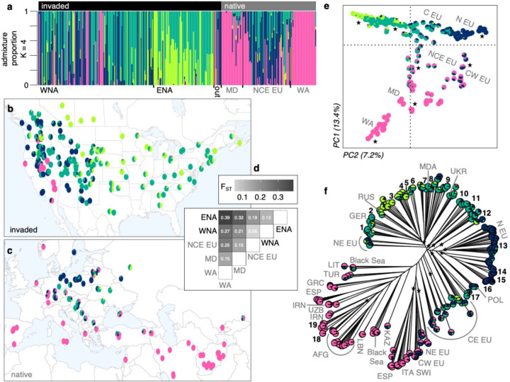
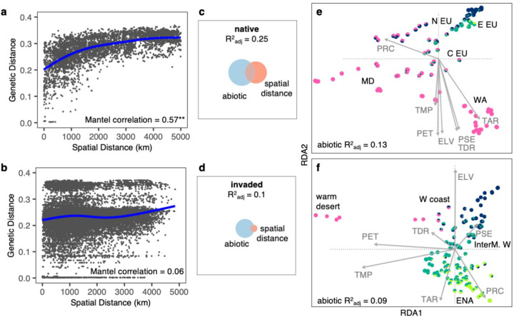
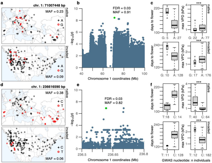
Local adaptation may facilitate range expansion during invasions, but the mechanisms underlying successful invasions remain unclear. Cheatgrass (Bromus tectorum), native to Eurasia and Africa, has invaded globally, with severe impacts in western North America. We aimed to identify mechanisms and consequences of local adaptation in the North American cheatgrass invasion. We sequenced 307 range-wide genotypes and conducted controlled experiments. We found that diverse lineages invaded North America, where long-distance gene flow is common. Nearly half of North American cheatgrass comprises a mosaic of ~19 locally adapted, near-clonal genotypes, each seemingly very successful in a different part of North America. Additionally, ancestry, phenotype, and allele frequency-environment clines in the native range predicted those in the invaded range, indicating pre-adapted genotypes colonized different regions. Common gardens showed directional selection on flowering time that reversed between warm and cold sites, potentially maintaining clines. In the USA Great Basin, genomic predictions of strong local adaptation identified sites where cheatgrass is most dominant. Our results indicate that multiple introductions and migration within the invaded range fueled local adaptation and success of cheatgrass in western North America. Understanding how environment and gene flow shape adaptation and invasion is critical for managing ongoing invasions.

Fig. 1:. The cheatgrass invasion involved multiple diverse introductions from the native range to North America

(a) Admixture proportions for K=4 ancestral genetic clusters (colors) for invasive and native genotypes in different regions; WNA: western North America (n=107), ENA: eastern North America (n=67), out: not in North America (n=8), MD: Mediterranean (n=24), NCE EU: north-central-east Europe (n=53), WA: west Asia (n=28). Geographic distribution of (b) invasive (n=194, North American only) and (c) native (n=105) genotypes. (d) Genetic differentiation (F_ST) between native and invaded regions, with notations following panel a. (e) Principal components analysis showing PC1 (y-axis) and PC2 (x-axis) explaining 20.6% of genomic variation. Axes are shifted to better reflect the latitudinal distribution of genotypes. Gray letters denote geographic origin in the native range and stars represent genotypes in the invaded range. (f) Neighbor-joining tree annotated with native (gray letters) and invaded locations (black numbers and stars). Native notations follow the ISO alpha-3 country code or their cardinal direction in Europe (EU). Black numbers mark groups of 2–14 near-clonal, and often widely distributed, invasive genotypes. Stars mark branches with invasive genotypes.

Fig. 2:. Genomic variation is structured by environment in the native and invaded ranges.

Strong isolation-by-distance in the (a) native (**Mantel p=10⁻⁴) but not in the (b) invaded range; plots show raw pair-wise data with a spline. Euler Plots show genomic variation is best explained by both the abiotic environment and spatial distance in (c) the native range, but only by the abiotic environment in (d) the invaded range. Fields of squares represent total genomic variation, circles represent genomic variation explained by a particular group of variables calculated using variance partitioning with RDA ordination (native n=105, invaded n=194). (e) Native and (f) invasive genotypes projected on the first two canonical axes of RDA (x-axis: RDA1 y-axis: RDA2). Arrows represent environmental predictors that strongly correlate with a maximal proportion of variation in linear combinations of SNPs. ELV: elevation, PET: potential evapotranspiration, PRC: total annual precipitation, PSE: precipitation seasonality, TAR: temperature annual range, TDR: temperature diurnal range, TMP: annual mean temperature. Colors are K=4 ancestral clusters. Geographic annotations are depicted in bolded black; N EU: north Europe, E EU: east Europe, C EU: central Europe, MD: Mediterranean, WA: west Asia, W coast: west coast, InterM. W: intermountain west, ENA: eastern North America.

Fig. 3:. Selection along aridity and temperature gradients shapes flowering phenology.

(a) Eigenvector plot with loadings of eleven phenotypes onto PC1 (x-axis) and PC2 (y-axis) describing axes of life history variation of 169 genotypes in a growth chamber; fl: Flowering, n: Number, inflor: Inflorescence. (b) Growth chamber phenotype-environment associations for invasive (left; n=138–145) and native genotypes (right; n=31–36). Coefficients of determination (R²), trends (gray lines), and 95% confidence intervals (gray shades) come from linear regressions. Significance comes from linear-mixed kinship models that accounted for relatedness among genotypes: *p<0.05, ***p<0.0001. (c) Fitness advantage of early flowering genotypes at a warm site/common garden (WI: Wild Cat, gray crosses, n=93) and of late flowering genotypes at a cool site/common garden (SS: Sheep Station, gray open circles, n=82) in two consecutive years (top: 2022 Spring harvest and bottom: 2023 Spring harvest). Trends (gray lines) and 95% confidence intervals (gray shades) come from linear regressions. Significance comes from linear-mixed kinship models of fitness (seed count for 2022 and inflorescence mass for 2023) in response to mean first day of flowering (fl), site, and their interaction (int): *p=0.006, **p<0.0006, ***p<0.00001. In all panels colors are K=4 ancestral clusters.

Fig. 4:. Environmental trends of two flowering time QTL are mirrored between native and invasive genotypes.

(a and d) Geographic distribution of QTL SNP alleles in the native (top) and invaded (bottom) range; crosses represent the reference/major allele, and open circles the alternate/minor allele. (b and e) Zoomed-in Manhattan plots showing Wald-test p-values (plotted as –log₁₀) from GWAS and genomic location of top SNP (marked in green), with respective false-discovery-rate (FDR) and minor allele frequency (MAF). (c and f) Phenotypic (boxplots to the left) and environmental variation (boxplots to the right) of flowering time QTL SNP alleles identified with GWAS. Boxplots indicate median (middle line), 25^th, 75^th percentile (box), and whiskers cover the data extent. ***p<0.0008 from two-tailed t-tests, but kinship linear-mixed models showed no significant differences. Max VPD: Maximum vapor pressure deficit in kPa. A, G, T, C on maps and x-axis of boxplots indicate nucleotides.

Fig. 5:. Genomic predictions of strong local adaptation occur in regions where cheatgrass is most dominant.

(a) Geographic distribution of the genomic offset estimated for each invasive genotype (n=194). The genomic offset or maladaptation is the genetic distance between observed invasive genotypes and the genotype-environment predictions in the invaded range based on the native range genotype-environment association. (b) Histograms of the mean genetic distance (offset) of 1000 null permutations in western North America (WNA, n=127) and eastern North America (ENA, n=67), relative to their estimated mean genetic distance (red lines). (c) Within the Great Basin (polygon in a, n=55), the mean genetic distance (offset) is significantly lower in areas where cheatgrass occurs in high (i.e., representing >15% vegetation cover) vs. low abundance. Boxplots indicate median (middle line), 25^th, 75^th percentile (box), and whiskers cover the data extent.

References

1. Daly E. Z. et al. A synthesis of biological invasion hypotheses associated with the introduction–naturalization–invasion continuum. Oikos 2023, e09645 (2023).
1. Catford J. A., Jansson R. & Nilsson C. Reducing redundancy in invasion ecology by integrating hypotheses into a single theoretical framework. Diversity and Distributions 15, 22–40 (2009).
1. Liu D. et al. Regional invasion history and land use shape the prevalence of non-native species in local assemblages. Glob. Chang. Biol. 30, e17426 (2024). - PubMed
1. Colautti R. I. & Barrett S. C. H. Rapid adaptation to climate facilitates range expansion of an invasive plant. Science 342, 364–366 (2013). - PubMed
1. Urban M. C. et al. Evolutionary origins for ecological patterns in space. Proc. Natl. Acad. Sci. 117, 17482–17490 (2020). - PMC - PubMed
Publication types
LinkOut - more resources