Neuronal wiring diagram of an adult brain

Abstract

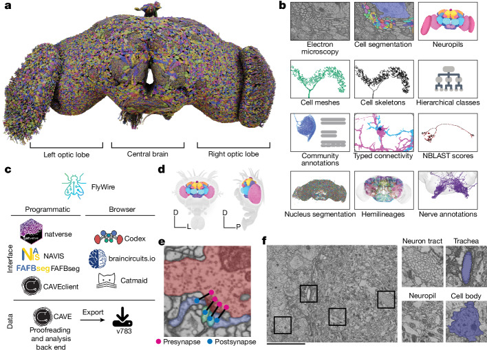
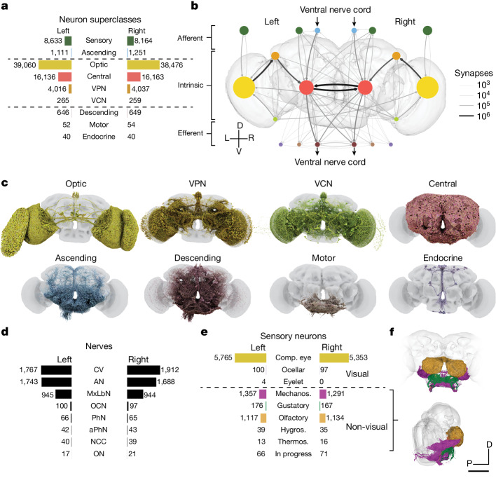
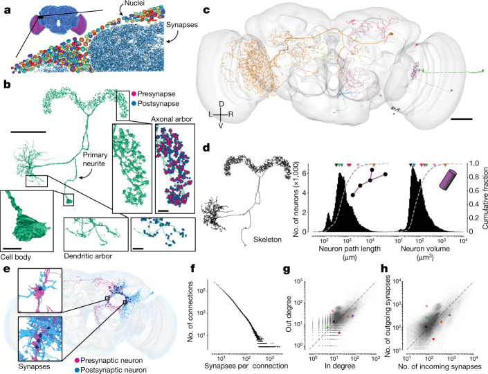
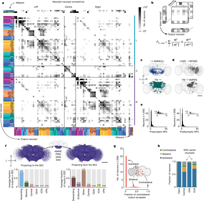
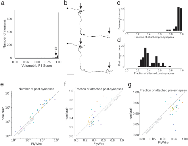
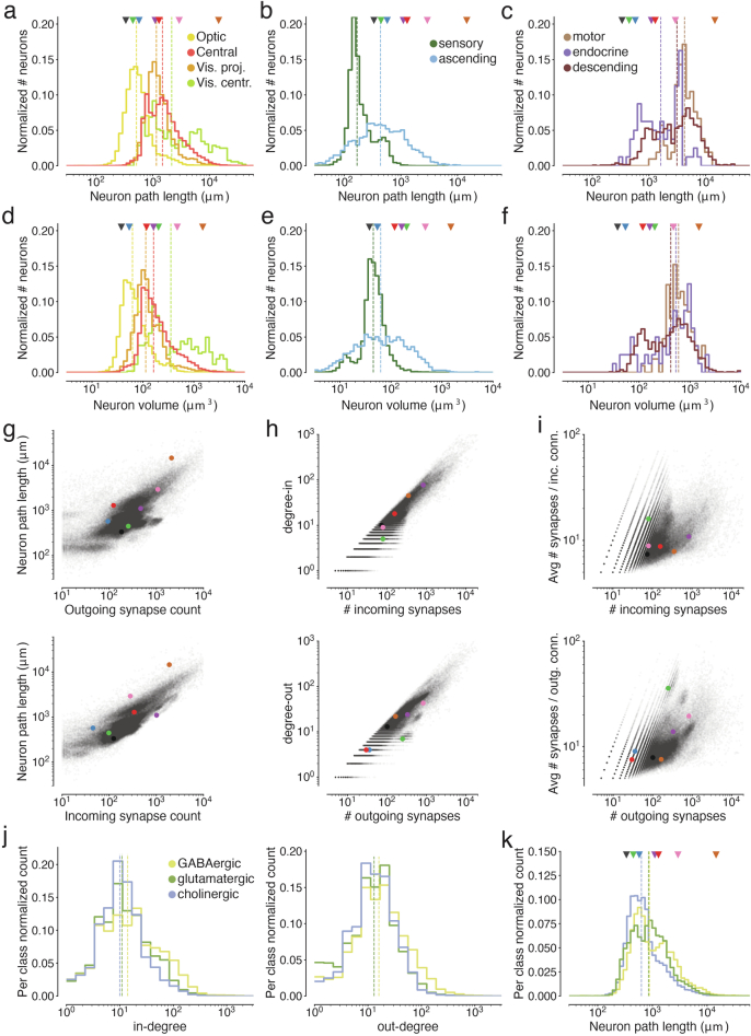
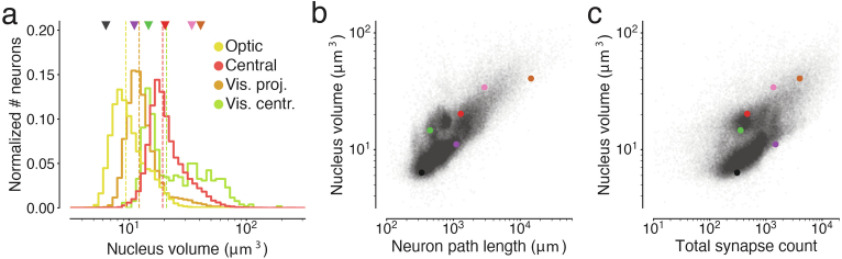
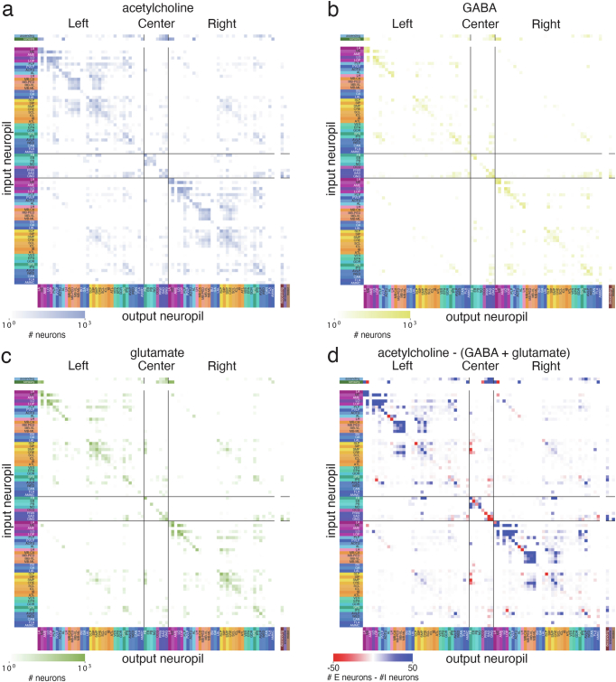
Connections between neurons can be mapped by acquiring and analysing electron microscopic brain images. In recent years, this approach has been applied to chunks of brains to reconstruct local connectivity maps that are highly informative^1-6, but nevertheless inadequate for understanding brain function more globally. Here we present a neuronal wiring diagram of a whole brain containing 5 × 10⁷ chemical synapses⁷ between 139,255 neurons reconstructed from an adult female Drosophila melanogaster^8,9. The resource also incorporates annotations of cell classes and types, nerves, hemilineages and predictions of neurotransmitter identities^10-12. Data products are available for download, programmatic access and interactive browsing and have been made interoperable with other fly data resources. We derive a projectome-a map of projections between regions-from the connectome and report on tracing of synaptic pathways and the analysis of information flow from inputs (sensory and ascending neurons) to outputs (motor, endocrine and descending neurons) across both hemispheres and between the central brain and the optic lobes. Tracing from a subset of photoreceptors to descending motor pathways illustrates how structure can uncover putative circuit mechanisms underlying sensorimotor behaviours. The technologies and open ecosystem reported here set the stage for future large-scale connectome projects in other species.

Fig. 1. A connectomic reconstruction of a whole fly brain.

a, All neuron morphologies reconstructed with FlyWire. All neurons in the central brain and both optic lobes were segmented and proofread. Note that image and dataset are mirror inverted relative to the native fly brain. b, An overview of many of the FlyWire resources that are being made available. FlyWire leverages existing resources for electron microscopy imagery by Zheng et al., synapse predictions by Buhmann et al. and Heinrich et al., and neurotransmitter predictions by Eckstein et al.. Annotations of the FlyWire brain dataset such as hemilineages, nerves and hierarchical classes are established in the accompanying paper. c, FlyWire uses CAVE for proofreading, data management and analysis back end. The data can be accessed programmatically through CAVEclient, navis, fafbseg and natverse, and through the browser in Codex, Catmaid Spaces and braincircuits.io. Static exports of the data are also available. d, The Drosophila brain can be divided into spatially defined regions based on neuropils (Extended Data Fig. 1). Neuropils for the lamina are not shown. D, dorsal; L, lateral; P, posterior. e, Synaptic boutons in the fly brain are often polyadic such that there are multiple postsynaptic partners per presynaptic bouton. Each link between a pre- and a postsynaptic location is a synapse. f, Neuron tracts, trachea, neuropil and cell bodies can be readily identified from the electron microscopy data acquired by Zheng et al.. Scale bar, 10 μm.

Fig. 2. Neuron categories.

a, We grouped neurons in the fly brain by ‘flow’: intrinsic, afferent or efferent. Each flow class is further divided into ‘superclasses’ on the basis of location and function. Neuron annotations are described in more detail in our companion paper. 201 neurons were not assigned to a hemisphere and are thus omitted from this panel. b, Using these neuron annotations, we created an aggregated synapse graph between the superclasses in the fly brain. D, dorsal; L, left; R, right; V, ventral. c, Renderings of all neurons in each superclass. d, There are eight nerves into each hemisphere in addition to the ocellar nerve and the cervical connective nerve. All neurons traversing the nerves have been reconstructed and accounted for. AN, antennal nerve; aPhN, accessory pharyngeal nerve; CV, cervical (neck) connective nerve; MxLbN, maxillary–labial nerve; NCC, nervii corpora cardiaca; OCN, ocellar nerve; ON, occipital nerve; PhN, pharyngeal nerve. e, Sensory neurons can be subdivided by the sensory modality that they respond to. Almost all sensory neurons have been typed by modality. The counts for the medial ocelli were omitted and are shown in Fig. 7b. Comp. eye, compound eye; hygros., hygrosensory; mechanos., mechanosensory; thermos., thermosensory. f, Renderings of all non-visual sensory neurons. Scale bar, 100 µm.

Fig. 3. Neuron and connection sizes.

a, The synapse-rich (synapses shown in blue) neuropil is surrounded by a layer of nuclei (random colours) located at the outside of the brain as well as between the optic lobes (purple) and the central brain (blue). b, An LPsP (lateral accessory lobe–posterior slope–protocerebral bridge) neuron can be divided into morphologically distinct regions. Synapses (purple and blue) are found on the neuronal twigs and only rarely on the backbone. c, We selected seven diverse neurons as a reference for d–h. d, The morphology of a neuron can be reduced to a skeleton (left) from which the path length can be measured. The histograms show the distribution of path length (middle) and volume (right; the sum of all internal voxels) for all neurons. The triangles on top of the distributions indicate the measurements of the neurons in c. e, Connections in the fly brain are usually multisynaptic, as in this example of neurons connecting with 71 synapses. f, The number of connections with a given number of synapses. g, In degree and out degree of intrinsic neurons in the fly brain are linearly correlated (R = 0.76). The dashed line is the unity line. Coloured dots indicate measurements of the neurons in c. h, The number of synapses per neuron varies between neurons by more than one order of magnitude and the number of incoming and outgoing synapses is linearly correlated (R = 0.81). Only intrinsic neurons were included in this plot. The dashed line is the unity line. Coloured dots indicate measurements of the neurons in c. Scale bars: 50 μm, b (main image) and c; 10 µm, b (expanded views).

Fig. 4. Neuropil projections and analysis of crossing neurons.

a, Whole-brain neuropil–neuropil connectivity matrix. The main matrix was generated from intrinsic neurons, and afferent and efferent neuron classes are shown on the side. Incoming synapses onto afferent neurons and outgoing synapses from efferent neurons were not considered for this matrix. See Extended Data Fig. 5 for neurotransmitter-specific matrices. Neuropils are defined in Extended Data Fig. 1. C, centre neuropils; L, left neuropils; R, right neuropils. b, Cartoon describing the generation of the matrix in a. The connectivity of each neuron is mapped onto synaptic projections between different neuropils. ${\mathbf{n}}_i^{\mathrm{out}}$ and ${\mathbf{n}}_i^{\mathrm{in}}$ are vectors of numbers of synapses for each neuropil and neuron. c,d, Examples from the matrix in a with each render corresponding to one row or column in the matrix (c) and examples from the matrix with each render corresponding to one square in the matrix (d). e, Most neurons have pre- and postsynaptic locations in fewer than four neuropils. Insets show a closer view of the long tail of the distribution. NPs, neuropils. f, Renderings (subset of 3,000 each) and input and output fractions of neurons projecting to and from the SEZ. The SEZ is composed roughly of five neuropils (the AMMC has left and right homologues). Average input and output fractions were computed by summing the row and column values of the SEZ neuropils in the superclass-specific projection matrices. g, Fraction of contralateral synapses for each central brain neuron. h, Fraction of ipsilateral, bilateral and contralateral neurons projecting to and from the centre neuropils per superclass. Scale bars, 100 µm.

Fig. 5. Optic lobes.

a, Rendering of a subset of the neurons in the fly brain. A cut through the optic lobe is highlighted and neuropils are annotated. b, A single Mi1 neuron (left) and all neurons that share a connection with the single Mi1 neuron (at least five synapses) (right). Three large neurons (CT1, OA-AL2b2 and Dm17) were excluded for the visualization. c, Top, Mi4, Dm12, Dm14 and Dm17 neurons in the right optic lobe, as annotated by Matsliah et al.. Bottom, expanded views of the outlined regions in Mi4 and Dm12 show the local structure. For Dm12, the right image shows a single neuron in black and all other Dm12 neurons are in background. d, The two LPi14 neurons in the right lobula plate (neuropil shown in background). Scale bars: 50 µm, b and c,d (main image); 10 µm, c,d (expanded views).

Fig. 6. Information flow through the Drosophila central brain.

a, We applied an information flow model for connectomes to the connectome of the central brain neurons. Neurons are traversed probabilistically according to the ratio of incoming synapses from neurons that are in the traversed set. The information flow calculations were seeded with the afferent classes of neurons (including the sensory categories). b, We rounded the traversal distances to assign neurons to layers. For gustatory neurons, we show a subset of the neurons (up to 1,000) that are reached in each layer. Neurons are coloured according to the traversal distance in c. c, UMAP analysis of the matrix of traversal distances, resulting in a 2D representation of each neuron in the central brain. Neurons from the same class co-locate (see also Extended Data Fig. 9). The small UMAP plots aligned with layers in b show where the neurons for each rank from the gustatory neurons fall within the distribution (black dots). Bottom, we coloured neurons in the UMAP plot by the rank order in which they are reached from gustatory seed neurons. Red neurons are reached earlier than blue neurons. LN, local neuron. d, As in c, bottom, for multiple seed neuron sets (see Extended Data Fig. 8c for the complete set). Mech. - JO, mechanosensory—Johnston’s organ. e, For each sensory modality, we used the traversal distances to establish a neuron ranking. Graphs show the distributions of neurons of each superclass within the specific rankings for each sensory modality (see Extended Data Fig. 8a for the complete set). f, Neurons were assigned to neurotransmitter types. Graphs show their distribution within the traversal rankings similar to d. Arrows highlight the sequence of GABA–glutamate peaks found for almost all sensory modalities (see Extended Data Fig. 8b for the complete set).

Fig. 7. Ocellar circuits and their integration with VPNs.

a, Overview of the three ocelli (left (L), medial (M) and right(R)) positioned on the top of the head. Photoreceptors from each ocellus project to a specific subregion of the ocellar ganglion which are separated by glia (marked with black lines on the electron micrograph (bottom)). Left and right are flipped in accordance with the orientation of the dataset (Methods). b, Renderings of the axons of the photoreceptors (left) and their counts (bottom right). Top right, location of the ocellar ganglion relative to the brain. c, Renderings of OCG01, OCG02 and DNp28 neurons with arbors. ‘Information flow’ from presynapses and postsynapses is indicated by arrows along the arbors. d, Connectivity matrix of connections between photoreceptors and ocellar projection neurons, including two descending neurons (DNp28). e, Comparison of number of glutamatergic and cholinergic synapses from ocellar projection neurons from the lateral eyes onto downstream neurons coloured by superclass (R = 0.78, P < 10⁻²⁶). f, Summary of the observed connectivity between ocellar projection neurons, VPNs and descending neurons. Scale bars, 100 µm.

Extended Data Fig. 1. Neuropils of the fly brain

.

Extended Data Fig. 2. Completeness and accuracy of FlyWire’s reconstruction.

(a) shows the result of our evaluation of proofread segments in the central brain. Experts attempted further proofreading of 826 neurons. We computed volumetric overlaps between the original and the final segment to calculate precision, recall, and F1 Scores. (b) Examples (top: before, bottom: after) of the changes made during further proofreading for a neuron scoring an F1-Score of 0.936. Arrows highlight locations that changed. (c,d) For each neuropil, we quantified what fraction of the synapses within it are pre- and postsynaptically attached to a proofread segment. (c) displays the distribution for presynaptic attachment and (d) the distribution for postsynaptic attachment. (e, f, g) Comparisons between FlyWire’s reconstruction and the hemibrain were made for overlapping neuropils. Dots represent neuropils and are colored according to Extended Data Fig. 1. (e) Comparison of the number of automatically detected synapses. The axes are log-transformed. (f) Comparison of post-synaptic completion rates and (g) pre-synaptic completion rate. The axes are truncated.

Extended Data Fig. 3. Measurements of neuron size.

Colored markers refer to neurons in Fig. 3b. Vertical dashed lines are medians. (a) Neuron path lengths of intrinsic neurons, (b) afferent neurons, and (c) efferent neurons by super-class. (d) Volumes of intrinsic neurons, (e) afferent neurons, and (f) efferent neurons by super-class. (g) Comparisons of path lengths and number of incoming and outgoing synapses. (h) For intrinsic neurons, comparisons of the in- and out-degrees with the number of incoming and outgoing synapses. Every dot is a neuron. (i) Comparison of average connection strengths (synapses per connection) with the number of synapses. Every dot is a neuron. (j) In- and out-degree distributions by neurotransmitter type. (k) Neuron path lengths by neurotransmitter type.

Extended Data Fig. 4. Measurements of neuron size.

Colored markers refer to neurons in Fig. 3b. Vertical dashed lines are medians. (a) Nucleus volume of intrinsic neurons, (b) Comparisons of nucleus volume and path length for intrinsic neurons and (c) nucleus volume and total synapse count.

Extended Data Fig. 5. Neuropil-neuropil projection maps.

(a) Projection maps produced as in Fig. 4a limited to connections from cholinergic, (b) GABAergic, and (c) glutamatergic neurons. (d) The difference between the putative excitatory (acetylcholine) and the putative inhibitory (GABA, glutamate) projection maps.

Extended Data Fig. 6. Neuropil-neuropil projections compared between hemispheres.

Each dot is a neuropil-neuropil projection in one hemisphere and the axes show the fractional weights as calculated in Fig. 4a,b. Red dots are comparisons between the same neuropils in different hemispheres (e.g. AMMC(L) -> VLP(L) vs AMMC(R) -> VLP(R). (a) Comparison of projections between neuropils in both hemispheres and between hemispheres. (b) Comparisons of projections with the center neuropils. (c) Comparisons of projections between ipsilateral and contralateral neuropil projections. (d) Comparisons of the distances between neuropil centroids with the fractional neuron weights. Connections within neuropils were excluded and neuropil pairs connected with <1 fractional neuron weight are not shown.

Extended Data Fig. 7. Input side analysis.

We assigned postsynaptic locations to either the center region or the left or right hemisphere. (a-g) For each super-class, (top plot). The lower plot shows the fraction of synapses in the center vs the lateral regions for all neurons. (h) Each neuron was assigned to the side where it received most of its inputs.

Extended Data Fig. 8. Percentile ranks for every modality.

(a) For each sensory modality (rows) we used the traversal distances to establish a neuron ranking. Each panel shows the distributions of neurons of each super-class within the sensory modality specific rankings. (b) Same as in (a) for the fast neurotransmitters. (c) Neurons in the central brain shown in the UMAP plot are colored by the rank order in which they are reached from a given seed neuron set. Red neurons are reached earlier than blue neurons.

Extended Data Fig. 9. Rank-based UMAP projection and neuropils.

(a) Every neuron in the central brain was assigned to the neuropil where it received the most synapses. Every dot is then colored by the assigned neuropil (see Extended Data Fig. 1 for neuropil colormap). (b) Same as in a but limited to the central complex neurons. Neurons in the central complex with an assigned neuropil other than the ones shown are colored black.

Extended Data Fig. 10. Ocellar circuit.

(a) Renderings of all neurons (excluding the photoreceptors) with arbors in the ocellar ganglion. “Information flow” from pre- and postsynapses is indicated by arrows along the arbors. (b) Overview of the three ocelli (left, medial, right) which are positioned on the top of the head. Photoreceptors from each ocellus project to a specific subregion of the ocellar ganglion which are separated by glia (marked with black lines on the EM). (c) Top view of the dendritic arbors within the ocellar ganglion of each DNp28 (brown) and OCG01 (blue: cholinergic, green: glutamatergic). The render on the lower shows all 12 OCG01s and 2 DNp28s. Each other render shows one neuron in color and all others in the background in gray for reference. (d) Comparison of number of synapses from OCG01 neurons and visual projection neurons onto descending neurons. (e) Connectivity matrix for connections between ocellar centrifugal neurons and ocellar projection neurons. (f) Inputs to ocellar centrifugal neurons by neuropil. Scale bars: 100 µm (a), 20 µm (c).

References

1. Scheffer, L. K. et al. A connectome and analysis of the adult Drosophila central brain. eLife9, e57443 (2020). - PMC - PubMed
1. Takemura, S.-Y. et al. A visual motion detection circuit suggested by Drosophila connectomics. Nature500, 175–181 (2013). - PMC - PubMed
1. Takemura, S., Nern, A., Chklovskii, D. B. & Scheffer, L. K. The comprehensive connectome of a neural substrate for ‘ON’ motion detection in Drosophila. eLife6, e24394 (2017). - PMC - PubMed
1. MICrONS Consortium. Functional connectomics spanning multiple areas of mouse visual cortex. Preprint at bioRxiv10.1101/2021.07.28.454025 (2021).
1. Shapson-Coe, A. et al. A petavoxel fragment of human cerebral cortex reconstructed at nanoscale resolution. Science384, eadk4858 (2024). - PMC - PubMed