Whole-brain annotation and multi-connectome cell typing of Drosophila

Abstract

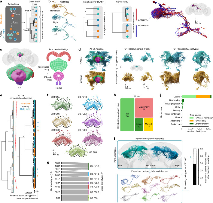
The fruit fly Drosophila melanogaster has emerged as a key model organism in neuroscience, in large part due to the concentration of collaboratively generated molecular, genetic and digital resources available for it. Here we complement the approximately 140,000 neuron FlyWire whole-brain connectome¹ with a systematic and hierarchical annotation of neuronal classes, cell types and developmental units (hemilineages). Of 8,453 annotated cell types, 3,643 were previously proposed in the partial hemibrain connectome², and 4,581 are new types, mostly from brain regions outside the hemibrain subvolume. Although nearly all hemibrain neurons could be matched morphologically in FlyWire, about one-third of cell types proposed for the hemibrain could not be reliably reidentified. We therefore propose a new definition of cell type as groups of cells that are each quantitatively more similar to cells in a different brain than to any other cell in the same brain, and we validate this definition through joint analysis of FlyWire and hemibrain connectomes. Further analysis defined simple heuristics for the reliability of connections between brains, revealed broad stereotypy and occasional variability in neuron count and connectivity, and provided evidence for functional homeostasis in the mushroom body through adjustments of the absolute amount of excitatory input while maintaining the excitation/inhibition ratio. Our work defines a consensus cell type atlas for the fly brain and provides both an intellectual framework and open-source toolchain for brain-scale comparative connectomics.

Fig. 1. Hierarchical annotation schema for a whole-brain connectome.

a, Hierarchical annotation schema for the FlyWire dataset (see the companion paper). Annotations for example cell type DA1 lPN (right) are highlighted in red. b, Renderings of neurons for each superclass. AN, antennal nerve; APhN, accessory pharyngeal nerve; CV, cervical connective; d, dorsal; m, medial; MxLbN, maxillary-labial nerve; NCC, corpora cardiaca nerves; OCG, ocellar ganglion; ON, occipital nerves; PhN, pharyngeal nerve; p, posterior. c, Annotation counts per field. Each colour within a bar represents discrete values; the numbers above bars count the discrete values. d, Left versus right neuron counts per superclass. Bottom, the left and right soma locations, respectively. e, Breakdown of sensory neuron counts into modalities. f, Flow chart of superclass-level, feed-forward (afferent to intrinsic to efferent) connectivity.

Fig. 2. Annotation of developmental units.

a, Illustration of the two complementary sets of annotations. b, Developmental organization of neuroblast hemilineages. c, Light-level image of an example AOTUv3 lineage clone; the lower case letters link canonical features of each hemilineage to the cartoon in b. Inset: cell body fibre tract in the EM. cb, cell body; np, neuropil. d, AOTUv3 neurons in FlyWire split into its two hemilineages. e, Cell body fibre bundles from all identified hemilineages, partially annotated on the right. f, The number of central brain neurons with an identified lineage; annotation of (putative (put.)) primary neurons is based on literature or expert assessment of morphology. g, The number of identified unique (hemi)lineages. h, Left versus right number of neurons contained in each hemilineage. i, Example morphological clustering of the AOTUv3 dorsal hemilineage reveals four distinct subgroups. j, Neurons belonging to the AOTUv3 dorsal hemilineage identified in the hemibrain connectome. k, FlyWire versus hemibrain number of neurons for cross-identified hemilineages.

Fig. 3. Across-brain stereotypy.

a, Schematic of the pipeline for matching neurons between FlyWire and the Janelia hemibrain connectomes. Conf., confidence. b, The distribution of top hemibrain to FlyWire NBLAST scores. c, Manual review for a sample of top NBLAST hits. d, The extrapolated number of hemibrain neurons with matches in FlyWire. e, Example for unlikely (left) and strong (right) morphology match. f, Example of a high-confidence cell type (PS008) that is unambiguously identifiable across all three hemispheres. g, Counts of FlyWire neurons that were assigned a hemibrain type. h, The number of hemibrain cell types that were successfully identified and the resulting number of FlyWire cell types. i,j, Examples for many:1 (i) and 1:many (j) hemibrain type matches. The dotted vertical lines indicate truncation of the hemibrain neurons. k, Graph representation of top NBLAST hits between FlyWire neurons and hemibrain types. This subgraph contains nodes within a radius of three edges from the query cell type (AVLP534). Neurons matching multiple cell types (asterisks) must be manually resolved, which is not always possible. l, The number of cells per cross-matched cell type within a brain (FlyWire left versus right) and across brains (FlyWire versus hemibrain).

Fig. 4. Connectivity stereotypy.

a, Connectivity comparisons and potential sources of variability. Reconstr., reconstruction. b, The number of pre- and post-synapses per cross-matched cell type. c,d, Edge weights (c) and cosine connectivity similarity (d) between cross-matched cell types. The whiskers represent 1.5× the interquartile range. e, The percentage of edges in one hemisphere that can be found in another hemisphere. f, The probability that an edge present in the hemibrain is found in one, both or neither of the hemispheres in FlyWire. A plot with normalized edge weights is shown in Extended Data Fig. 6d. g, The probability that an edge is found within and across brains as a function of total (left) and normalized (right) edge weight. The second x axis shows the percentage of synapses below a given weight. h, Correlation of across-edge (left) and within-edge (right) edge weights. The envelopes represent quantiles. i, Model for the impact of technical noise (synaptic completion rate, synapse detection) on synaptic weight from cell types i to j. The raw weight from the connectome for each individual edge is scaled up by the computed completion rate for all neurons within the relevant neuropil; random draws of the same fraction of those edges then allow an estimate of technical noise. j, Observed variability explainable by technical noise as fraction of FlyWire left–right edge pairs that fall within the 5–95% quantiles for the modelled technical noise. k, Modelled biological variability (observed variability − technical noise). R (b and c) is the Pearson correlation coefficient. For d, statistical analysis was performed using unpaired t-tests; ***P < 0.001.

Fig. 5. Variability in the mushroom body.

a, Schematic of mushroom body circuits. K refers to the number of ALPN types that a KC samples from. Neuron types not shown are as follows: DANs, DPM and OANs. b, Rendering of KC types. c, Per-type KC counts across the three hemispheres. d, KC post-synapse counts, normalized to total KC post-synapses in each dataset. e, The fraction of ALPN to KC budget spent on individual KC types. f, The number of ALPN types a KC receives input from K. The dotted vertical lines represent the mean. g, The fraction of APL to KC budget spent on individual KC types. h, The normalized excitation/inhibition ratio for KCs. An explanation of enhanced box plots is provided in the Methods. i, The fraction of MBON input budget coming from KCs. Each line represents an MBON type. j, MBON09 as an example for KC to MBON connectivity. All MBONs are shown in Extended Data Fig. 7. k, Dimensionality (dim(h)) as function of a modelled K. The arrowheads mark observed mean K values. l, Summarizing schematic. Exc., excitatory. For f and h, Cohen’s d effect size values are shown for pairwise comparisons where P ≤ 0.01; Welch’s tests (f) and Kolmogorov–Smirnov tests (h) were applied.

Fig. 6. Across-brain cell typing.

a, Cell type is defined as a group of neurons that are each more similar to a group in another brain than to any neurons in the same brain. We expect cell type clusters to be balanced, that is, contain neurons from all three hemispheres in approximately even numbers. b, Example of a hemibrain cell type (AOTU063) that is morphologically homogeneous but has two cross-brain consistent connectivity types and can therefore be split. c, Main neuropils making up the central complex (CX). d, Overview of all CX cells (left) and two subsets of fan-shaped body (FB, dotted outlines) cell types: FC1–3 and FB1–9 (right). e, Hierarchical clustering from connectivity embedding for FC1–3 cells. A magnification of cross-brain cell type clusters is shown. The asterisk marks a cluster that was manually adjusted. f, Renderings of FC1–3 across-brain types; the FB is outlined. The tiling of FC1–3 neurons can be discerned. g, Comparison of FC1–3 hemibrain and cross-brain cell types. The colours correspond to those in f. h, Mappings between hemibrain and cross-brain cell types for FB1–9. A detailed flow chart is provided in Extended Data Fig. 8. i, The pipeline for generating types for neurons without a hemibrain cell type. Hemilineage LHl2 dorsal is shown as an example. The box plot shows the fraction of FlyWire neurons with a hemibrain-derived cell type. j, Cell type source broken down by super class.

Extended Data Fig. 1. Completion of the FlyWire whole-brain connectome and cell typing reveal a left-right inversion of EM image data during acquisition of the underlying FAFB EM dataset.

A Frontal views of the adult fly brain are by convention shown in 2D projection, placing the fly’s right on the left of the page. In this view, the asymmetric body (AB), which is nearly always larger on the fly’s right^–, therefore appears on the left of the page (left panel). During acquisition of the FAFB dataset, image mosaics were acquired and inadvertently stored to disk with the left-right axis inverted. Therefore in frontal view, the right side of the FAFB/FlyWire brain, and the larger AB, appear on the viewer’s right (right panel). Insets show axons of SA1-3 neurons, which form the major input to the AB. B Direct examination of an original EM-imaged grid using differential interference contrast (DIC) microscopy and an acquired EM mosaic in neuroglancer/catmaid confirms a left-right inversion during image acquisition. A grid with a crack in the support film and staining artefact precipitate was selected in order to provide fiducials easily visible by light microscopy (left panel). These same artefacts can be seen in the EM mosaic (right panel). C Showcase of how to programmatically correct the inversion of FAFB/FlyWire data. Due to the large size of the original and derived datasets, it was not technically practical to correct the left-right inversion once it was detected. Therefore this must be corrected post hoc. Code samples show how this can be done for e.g. mesh or skeleton data using Python or R (Methods, “FAFB Laterality”).

Extended Data Fig. 2. Hierarchical annotation examples.

A Examples for cell class annotations. B Examples for labels derived from the hierarchical annotations. Abbreviations: ALRN, antennal lobe receptor neuron; MBON, mushroom body output neuron; ALLN, antennal lobe local neuron; ORN, olfactory receptor neuron; AN, antennal nerve.

Extended Data Fig. 3. Hemilineage atlas.

Anterior views of neurons within a hemilineage (based on^,), or neurons whose cell bodies form a cluster in a lineage clone (also referred to as “hemilineages” hereafter), based on the light-level data from^–,. The names of the hemilineages are at the bottom of each panel (top: Hartenstein nomenclature; bottom: ItoLee nomenclature). The snapshots only include neurons with cell bodies on the right hemisphere, and the central unpaired lineages. Except for the hemilineages that tile the optic lobe, the neurons are coloured by morphological groups (see Methods, Hemilineage annotations section). The neurons that form cohesive tracts with their cell body fibres in the Type II lineages (see Methods) are at the lower part of the panels. The last panel of the “Type II’ section is for orientation purposes. The bottom right panel is a histogram of the number of morphological groups per hemilineage (blue: hemibrain; orange: FlyWire right; green: FlyWire left). Inset is the number of neurons per hemisphere in each morphological group, with points coloured by their density (yellow: denser). Corresponding group names, together with FlyWire and neuroglancer links are available in Supplementary Files 2 and 3.

Extended Data Fig. 4. Across-brain neuron matching.

A Distribution of the fraction of each FlyWire neuron’s cable that is contained within the hemibrain volume: 1 = fully contained; 0 = entirely outside the volume. Note that where necessary FlyWire neurons were transformed onto the opposite side of the brain to better overlap with the hemibrain. B Distribution of top FlyWire → hemibrain NBLAST scores. C Top NBLAST score vs fraction of neuron contained within hemibrain volume. In a fraction of cases, even heavily truncated neurons can produce good scores and be successfully matched. D Top: distribution of top NBLAST scores and fraction which was type matched. Bottom: probability that the correct hit was the top NBLAST hit (green) or at least among (yellow) the top 10% as a function of the top NBLAST score. E When some FlyWire neurons had good NBLAST matches against multiple hemibrain cell types, we cross-compared within-dataset morphological clustering (dendrograms). We tried to assign hemibrain types to those ambiguous FlyWire neurons to exactly match clusters in the two dendrograms (“easy case”). When this failed because a cluster in the dendrogram contained clear matches to >1 hemibrain types, we merged types (“hard case”). F Cross-brain NBLAST co-clustering for example cell types in Fig. 3: SIP078/SIP080 (left) and PS090 (right). All hemibrain neurons are truncated. The FlyWire PS090 neurons (2 per hemisphere, none truncated) split into two well-separated clusters each containing one left and one right neuron, suggesting that the hemibrain cell type should be split. This is not the case for SIP078/SIP080 where the dendrogram cannot be split into subclusters containing neurons from each hemisphere. G Counts for 1:many and many:1 type matches. These also include types derived from previously untyped hemibrain neurons. H Extended version of NBLAST hit graph from Fig. 3k. Here, grey dotted arrows indicate matches to types outside of the displayed subgraph. I Fraction of cell types showing a difference in cell counts within (left/right, top) and across (bottom) brains. J Distribution of cell count differences. K Robust linear regression (Huber w/ intercept at 0) for within- and across-dataset pre/postsynapse counts from Fig. 3h. L Same data as in K but separated by superclass. Slopes are generally close to 1: 1.021 (pre-) and 1.035 (postsynapses, i.e. inputs) between the left and right hemisphere of FlyWire, and 1.176 (presynapses, i.e. outputs) 0.983 (post) between FlyWire and the hemibrain. Note that correlation and slope are noticeably worse for cell types known to be truncated such as visual projection neurons which suggests that we did not fully compensate for the hemibrain’s truncation and that the actual across-brain correlation might be even better.

Extended Data Fig. 5. Examples of biological outliers and sample artefacts.

A LC6 and LC9 neurons (lineage VPNd3) of the right and left hemispheres take different routes in FlyWire to equivalent destinations (previously reported in). Mushroom body (MB) peduncle is shown in pink. B Example of a left/right neuron pair where one side has extra dorsal and smaller ventral dendrites (red arrowheads). C A TuBu neuron (black) with correctly placed axon but misplaced ventral dendrites. Regular TuBu neurons shown in background for reference. D A single Kenyon Cell whose axon projects outside of the mushroom body, descending through the medial antennal lobe tract. E Cell type (CB1029, DM6 ventral hemilineage) where the left neurons’ dendrites (red) take a different tract. F Example of sample artefact: the axon of the left DM3 adPN has very dark cytosol which affects both the neuron segmentation as well as synapse detection. Insets compare two locations along the axons between the left and right neurons. G A subset of neurons from the ALl1 ventral hemilineage where the right neurons are missing their entire dendrites (red arrow). The exact reason for this is unknown but it is not due to insufficient proofreading. H Quantification of recorded outliers and sampling artefacts broken down by super class. Total number of neurons (left) as well as fraction (right) are shown. The number of biological outlier neurons is ~0.4% of the total number of neurons in the brain.

Extended Data Fig. 6. Across-brain connectivity.

A Comparison of normalized edge weights within (left) and across (right) brains. B Connectivity cosine connectivity similarity within and across brains. Each datapoint is a cell type identified across the three hemispheres. Size correlates with the number of cells per type. C Connectivity cosine similarity separated by neurotransmitter. Error bars represent the 95% CI. D Probability that an edge present in the hemibrain is found in one, both or neither of the FlyWire hemispheres. E Fraction of synapses contained in edges above given absolute (left) and normalized (right) weight. Horizontal lines mark the thresholds for a 90% chance that an edge is found in another hemisphere. F Postsynaptic completion rates. Each datapoint is a neuropil.

Extended Data Fig. 7. Across-brain mushroom body comparison.

A Graph showing ALPN/APL → KC connectivity across the three datasets. Edge labels provide weights both as total synapse counts and normalized to the total output budget of the source. In FlyWire, the mushroom bodies (MB) have 57.2% (left) and 60.7% (right) postsynaptic completion rate while the hemibrain MB has been proofread to 81.3% (see also B). To compensate for this we typically used normalized synapse counts and edge weights. Note that KCab act as an internal control as their numbers are consistent across all hemispheres and we don’t expect to see any changes in their connectivity. B Total versus proofread postsynapse counts across MB compartments. Lateral horn (LH) shown for comparison. C Postsynapse density across MB compartments. D Connectivity between different MB cell classes. Inset shows an example of KC → KC and KC → MBON synapse in the hemibrain. E Presynapse counts per KC type normalized to the total number of KC synapses per dataset. F ALPN → KC edge weights. See Methods for details on enhanced box plots. G K (# of ALPN types providing input to a single KC) under different synapse thresholds. H Fraction of MBON input budget coming from individual KCab, KCg-m and KCa’b’. Abbreviations: CA, calyx; DAN, dopaminergic neuron; ALPN, antennal lobe projection neuron; KC, Kenyon Cell; MBON, mushroom body output neurons. Kolmogorov-Smirnov test (F): *, p < =0.05; **, p < =0.01; ***, p < =0.001.

Extended Data Fig. 8. Across-brain co-clustering.

A FC1-3 across-brain cluster from Fig. 6d (asterisk) that was manually adjusted. This group consists of three sub-clusters that technically fulfil our definition of cell type. They were merged, however, because they individually omit columns of the fan-shaped body (arrowheads) and are complementary to each other. B Hierarchical clustering from combined morphology + connectivity embedding for FB1-9. Zoom-in shows cross-brain cell type clusters. C Number of hemibrain vs cross-brain FB1-9 cell types. D Examples from the FB1-9 cross-brain cell typing. Labels are composed from CB.FB{layer}{hemilineage-id}{subtype-id}; fan-shaped body outlined. E Flow chart comparing FB1-9 hemibrain and cross-brain cell types. Colours correspond to 1:1, 1:many, many:1 and many:many mappings between hemibrain and cross-brain cell types. F Renderings of all FB1-9 cross-brain cell types.

Extended Data Fig. 9. Double vs triple co-clustering analyses.

A Pipeline for comparing putative cell types from double (FlyWire left/right) and triple (FlyWire + hemibrain) hemisphere co-clustering. B Flow chart for hemilineage LHl2 dorsal illustrating how individual FlyWire neurons move between double and triple clusters. Black bars represent clusters; thickness is proportional to the number of neurons in each cluster. C Summary over all 25 hemilineages that were cross-identified and are untruncated in the hemibrain connectome. Top bar chart shows unfiltered results; bottom chart shows results after denoising (removal of single neurons that cause many:many mapping because they swap clusters). D Flow chart for example hemilineage SIPa1 ventral. Unfiltered (top) and denoised (bottom). E-F Example of a cluster (red in panel F) from hemilineage SLPa&l1 lateral that only seems to exist in FlyWire although similar balanced clusters (black) are present in both datasets.

Extended Data Fig. 10. CATMAID spaces.

Screenshot demonstrating the use of CATMAID Spaces (https://fafb-flywire.catmaid.org/) to interrogate the FlyWire connectome. Differential inputs to AOTU63a and b are visualized (red and cyan, respectively). The Graph widget was used to show all neurons making 20 or more synapses onto AOTU63a and b, and to show only >=20 synapse connections between these neurons. Neurons whose only >=20 synapse connection was to either AOTU63a or b (but not both) were differentially coloured (blue-purples and greens, respectively).

Extended Data Fig. 11. Annotations in Neuroglancer.

A Screenshot of neuroglancer with FlyWire 783 segmentation layer with “flytable-info-783” annotation layer subsource (scene pre-configured at http://tinyurl.com/flywire783). B Example for querying annotation. C Example for subsource “flytable-info-783-all” which includes hemilineage annotations.

Extended Data Fig. 12. Matching workflow.

A Workflow for matching hemibrain types to FlyWire neurons. B Workflow for generation of de-novo cell types used to fill the gaps left from the hemibrain type matching. C Workflow for cell typing in the optic lobes. D-G Examples of cell types. H2 is based on left vs right FlyWire clustering plus existing LM data; DNge139 and CB592 are based solely on left vs right FlyWire clustering; DNa01 is based on three hemispheres worth of data but was misidentified as “VES006” in the hemibrain.

References

1. Dorkenwald, S. et al. Neuronal wiring diagram of an adult brain. Nature10.1038/s41586-024-07558-y (2024). - PMC - PubMed
1. Scheffer, L. K. et al. A connectome and analysis of the adult central brain. eLife9, e57443 (2020). - PMC - PubMed
1. White, J. G., Southgate, E., Thomson, J. N. & Brenner, S. The structure of the nervous system of the nematode Caenorhabditis elegans. Philos. Trans. R. Soc. Lond. B314, 1–340 (1986). - PubMed
1. Varshney, L. R., Chen, B. L., Paniagua, E., Hall, D. H. & Chklovskii, D. B. Structural properties of the Caenorhabditis elegans neuronal network. PLoS Comput. Biol.7, e1001066 (2011). - PMC - PubMed
1. Abbott, L. F. et al. The mind of a mouse. Cell182, 1372–1376 (2020). - PubMed
Publication types