Neuronal parts list and wiring diagram for a visual system

Abstract

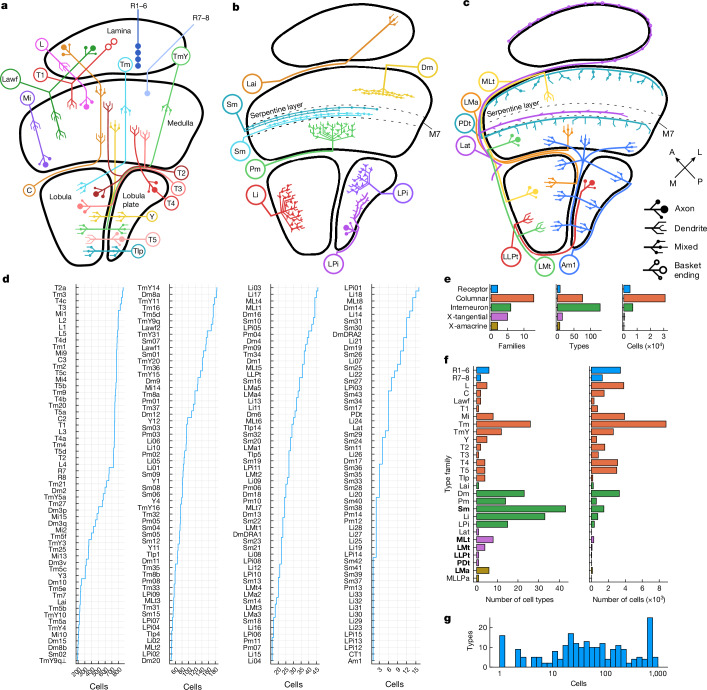
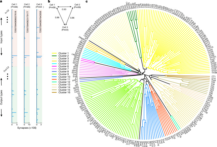
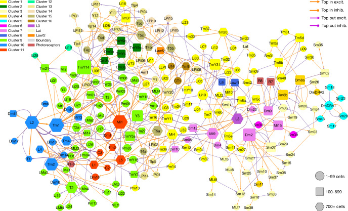
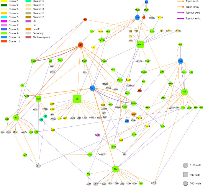
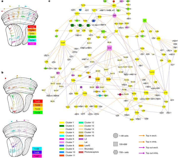
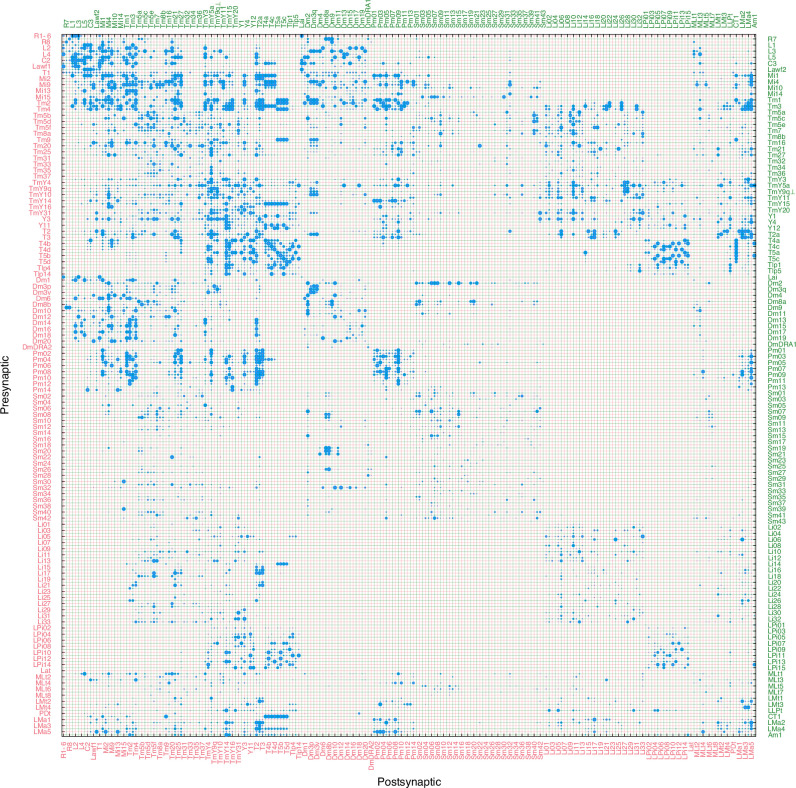
A catalogue of neuronal cell types has often been called a 'parts list' of the brain¹, and regarded as a prerequisite for understanding brain function^2,3. In the optic lobe of Drosophila, rules of connectivity between cell types have already proven to be essential for understanding fly vision^4,5. Here we analyse the fly connectome to complete the list of cell types intrinsic to the optic lobe, as well as the rules governing their connectivity. Most new cell types contain 10 to 100 cells, and integrate information over medium distances in the visual field. Some existing type families (Tm, Li, and LPi)^6-10 at least double in number of types. A new serpentine medulla (Sm) interneuron family contains more types than any other. Three families of cross-neuropil types are revealed. The consistency of types is demonstrated by analysing the distances in high-dimensional feature space, and is further validated by algorithms that select small subsets of discriminative features. We use connectivity to hypothesize about the functional roles of cell types in motion, object and colour vision. Connectivity with 'boundary types' that straddle the optic lobe and central brain is also quantified. We showcase the advantages of connectomic cell typing: complete and unbiased sampling, a rich array of features based on connectivity and reduction of the connectome to a substantially simpler wiring diagram of cell types, with immediate relevance for brain function and development.

Fig. 1. Class, family, type and cell.

a, Families in the columnar class. C, centrifugal; L, lamina monopolar; Lawf, lamina wide-field; Mi, medulla intrinsic; R, receptor; T1–T5, T neuron; Tm, transmedullary; TmY, transmedullary Y; Tlp, translobula plate; Y, Y neuron. b, Families in the interneuron class. Serpentine medulla (Sm) is new. Dm, distal medulla; Lai, lamina intrinsic;  Li, lobula intrinsic, LPi, lobula plate intrinsic; Pm, proximal medulla. c, Families in the cross-neuropil tangential and amacrine classes. For tangential families, axon and dendrite are distinguished graphically. All are new except for Lat and Am1. LLPt, lobula–lobula plate tangential; LMt, lobula–medulla tangential; LMa, lobula medulla amacrine; Lat, lamina tangential; MLt, medulla–lobula tangential; PDt, proximal to distal medulla tangential. A, anterior; L, lateral; M, medial; P, posterior. d, Cell types are ordered by the number of proofread cells in each type, starting with the most numerous types. Additional details are provided in Extended Data Tables 1 and 2. e, The numbers of families (left), types (middle) and cells (right) in each class. f, The numbers of types (left) and cells (right) in each neuropil-defined family. Bold font indicates families that are entirely new, or almost entirely new. MLLPa, medulla lobula lobula plate amacrine, is a synonym for Am1. g, The number of types versus the number of cells in a type. The x axis denotes type size (log-scale), and the y axis shows the number of types with matching size. The peak near 800 consists of the numerous types—those with approximately the same cardinality as the ommatidia of the compound eye.

Fig. 2. Clustering of cells and cell types based on connectivity.

a, Feature vectors for three example cells. The horizontal axis indicates the synapse numbers that the cell receives from presynaptic types (red region of vertical axis) and sends to postsynaptic types (green region of vertical axis). Cells 1 and 2 (same type) have more similar feature vectors to each other than to cell 3 (different type). The long numbers are the cell IDs in version 783 of the FlyWire connectome. b, Cells 1 and 2 (same type) are closer to each other than to cell 3 (a different type), according to the weighted Jaccard distances between the cell feature vectors. Such distances are the main basis for dividing cells into cell types (Methods). c, Dendrogram of cell types. Cell types that merge closer to the circumference are more similar to each other. Flat clustering (16 colours) is created by thresholding at 0.9. A few clusters containing single types (Lat, L3 and Lawf2) are uncoloured. To obtain the dendrogram, feature vectors of cells in each type were summed or averaged to yield a feature vector for that cell type, and then cell type feature vectors were hierarchically clustered using average linkage. Jaccard distances run from 0.4 (circumference) to 1 (centre). Clusters containing more than one cell type (legend with coloured lines) are numbered starting at ‘3 o’clock’ on the dendrogram and proceeding counterclockwise. Source Data

Fig. 3. Wiring diagram of cell types—top input and output connections.

Simplified wiring diagram of all cell types intrinsic to the optic lobe and photoreceptors, showing only the top input and output connections of each type. Colours of types (nodes) indicate membership in flat clusters of Fig. 2c. The node size encodes the number of drawn connections, so that hub types look larger. The node shape encodes type numerosity (number of cells). The line colour encodes the relationship (top input versus top output) and the line width is proportional to the number of synapses. The line arrowhead shapes encode excitation (excit.) versus inhibition (inhib.). Further explanation is provided in the Methods.

Fig. 4. ON, OFF and luminance channels—top inputs and outputs only.

Simplified wiring diagram of ON (cluster 11, red), OFF (cluster 10, blue) and luminance (cluster 7, violet and L3) channels and their primary connections with other subsystems and VPNs. For clarity, only the top input and output connections are shown for each type. Further explanation is provided in Fig. 3 and the Methods.

Fig. 5. Motion subsystem—top inputs and outputs only.

a, Cell types of the motion subsystem (clusters 13 to 16) and their primary connections with other subsystems and VPNs. The motion-detecting T4 types are located at the corners of the square layout, and often share postsynaptic targets with the corresponding T5 types. TmY14 is the top output of many types. For clarity, only the top input and output connections are shown for each type. Further explanation is provided in Fig. 3 and the Methods. b, LPi14, also called LPi1-2, is a jigsaw pair of full-field cells. c, LPi02 stratifies in the same lobula plate layers as LPi14, but the cells are smaller. d, LPi08 is an example of an interneuron that is not amacrine. It is polarized, with a bouton-bearing axon that is dorsally located relative to the dendrite. D, Dorsal. Scale bar, 30 μm.

Fig. 6. Hypothetical object subsystem.

Cell types of the object subsystem (clusters 9 and 12) and their primary connections with other subsystems and VPNs. T2 and T3 are known to be activated by small objects. For clarity, only the top input and output connections are shown for each type. Further explanation is provided in Fig. 3 and the Methods.

Fig. 7. Hypothetical colour subsystem.

a, Tm5a to Tm5c correspond with types that were previously defined by molecular means. Tm5d to Tm5f have similar morphologies, but different connectivity patterns (Supplementary Data 5). b, Tm31 to Tm37 are new members of the Tm family that project from the serpentine layer (M7) to the lobula. c, Cell types in the colour subsystem (clusters 1, 3 and 4) and their top connections with other subsystems and VPNs. For clarity, only the top input and output connections are shown for each type. Further explanation is provided in Fig. 3 and the Methods.

Fig. 8. Morphological variation.

a, Typical TmY14 cells (cyan) have axonal projections to the central brain (left). Atypical cells (red) initially project toward the central brain, but their axons turn around and terminate in the medulla. As the axons bear few synapses, typical and atypical cells are approximately the same in connectivity. b, Representative typical (cyan) and atypical (red) TmY14 with an axon projecting into the central brain (cyan arrow) and medulla (red arrow), respectively. c, Typical Tlp4 cells arborize in the lobula plate and lobula. A few cells (pseudo-Y11) have an additional branch in the medulla (right), and resemble Y11 cells in morphology but have the same connectivity as Tlp4. d, Relative to a typical Tlp4 cell (red), a pseudo-Y11 cell (blue) has an additional branch in the medulla. e, Li11 does not project into the central brain. f, Pseudo-Li11 has an additional arbour projection into the central brain. This arbour makes a few synapses, and might lead to the conclusion that pseudo-Li11 should be categorized as Li11. However, the connectivity between Li11 and pseudo-Li11 is fundamentally different, making them distinct types. Scale bar, 30 µm.

Fig. 9. Different kinds of spatial coverage.

a, Dm4 has full spatial coverage, and tiles perfectly with no overlap. b, Dm dorsal rim area 2 (DmDRA2) covers the dorsal rim. c, Sm05 covers the dorsal hemifield. d, Sm01 covers the ventral hemifield. e, Sm33 are H-shaped cells that cover the anterior and posterior rim. f, Sm39 is a single cell with mixed coverage: dorsal dendritic arbour in M7 and full-field axonal arbour in M1. V, ventral. Scale bar, 50 μm.

Extended Data Fig. 1. Cell counts of types in optic lobe versus central brain.

a, Drosophila central brain and flanking optic lobes. Neurons intrinsic to the optic lobes (colours) are the subject of this study (A: Anterior. L: Lateral. D: Dorsal). b, Boundary cells straddle the optic lobe and central brain (H: heterolateral, VCN: visual centrifugal neuron: VPN: visual projection neuron). c, Optic lobe main neuropils (brain regions) and their layering (A: Anterior. L: Lateral. M: Medial. P: Posterior). d, Distribution of number of optic lobe types by bucketed unilateral cardinality. Each bar represents types whose cardinality (number of cells) is within the specified range. Most types contain 10+ cells, and a significant portion of types contain hundreds of cells. e, Distribution of the number of central brain types by bucketed bilateral cardinality. In contrast to the optic lobe, here most types have cardinality 2 (cell and its mirror twin in the opposite hemisphere).

Extended Data Fig. 2. Logical connectivity predicate statistics.

a, Number of types by predicate F-score range. b, Number of cells by their types’ predicate F-score range. c, Number of types by predicate size, that is the sum of the number of input features and output features participating in the binary conjunction. d, Number of cells by their types’ predicate size.

Extended Data Fig. 3. Discrimination in high and low dimensions.

a, Radii of types in high-dimensional feature space. b, Histogram of type radii in high-dimensional feature space. c, Example 2D discriminator for Pm04 cells (red) versus other Pm types (blue). On the X and Y axis are the fraction of their inputs/outputs in C3 / TmY3 respectively.

Extended Data Fig. 4. Type-to-type connectivity as a matrix.

The number of synapses from one cell type to another is indicated by the area of the corresponding dot. Dot area saturates above 3600 synapses, to make weaker connections visible. For legibility, the type names alternate between left and right edges, and bottom and top edges, and are colour coded to match the lines that are guides to the eye.

Extended Data Fig. 5. Wiring diagram of cell types (top input connections).

Wiring diagram depicting top inputs for all cell types intrinsic to the optic lobe, as well as photoreceptors. Node size encodes the number of drawn connections, highlighting “hub” inputs. Node colour indicates membership in the subsystems defined in the text. See legend and additional explanation in Fig. 3 and Methods.

Extended Data Fig. 6. Wiring diagram of cell types (top output connections).

Wiring diagram depicting top outputs for all types intrinsic to the optic lobe. Node size encodes the number of drawn connections, highlighting “hub” outputs. Node colour indicates membership in the subsystems defined in the text. See legend and additional explanation in Fig. 3 and Methods.

Extended Data Fig. 7. Input and output perplexity.

a, Input (blue) and output (red) perplexities. Types are ordered by the product of input and output perplexities. b, Output and input perplexity are correlated. Out-perplexity tends to exceed in-perplexity (more points above red line drawn to indicate equality of out and in).

Extended Data Fig. 8. Difference between output and input entropies.

The difference between output and input entropies (units of nats) quantifies the degree of divergence or convergence. This difference is equivalent to the logarithm of the ratio of out- and in-perplexities. The connectivity of the top types (top left) is more divergent, as the output entropy is greater than the input entropy. The connectivity of the bottom types (bottom right) is more convergent, as the input entropy is greater than the output entropy.

Extended Data Fig. 9. Comparison with seven-column reconstruction.

We compared the synapse counts between type pairs to the corresponding synapse counts in the seven-column reconstruction. The types included in the reconstruction are: C2, C3, L1, L2, L3, L4, L5, Mi1, Mi4, Mi9, R7, R8, T1, T2, T2a, T3, Tm1, Tm2, Tm20 and Tm9. For this comparison we used the centre column and its surrounding 6 columns from our dataset (green dots) as well as the average of 100 columns and their surrounding ones (red dots). Each point represents an ordered pair of types, and the number of synapses between them in the FlyWire connectome (X) and the seven-column reconstruction (Y). Correlation coefficients are 0.952 for the centre + 6 columns and 0.954 for the average.

Extended Data Fig. 10. Carving the dendrogram to yield finer clusters.

The hierarchical clustering was coloured in Fig. 2c to indicate 19 flat clusters at a threshold of 0.9. (a) Lowering the threshold to 0.885 yields 26 clusters (b) Lowering the threshold further to 0.86 yields 36 clusters. Clusters containing a single cell type are uncoloured (black). R1-6 and L3 are separate clusters in both panels.

Extended Data Fig. 11. Wiring diagram of type clusters (major input and output connections).

a, Wiring diagram depicting major input and output connections between type clusters of Fig. 2c. Node size encodes the number of drawn connections. For each cluster major inputs are drawn as orange inbound edges, and major outputs as purple outbound edges. Major input/output connection is defined as having at least 50% synapses relative to top input/output connection respectively, excluding loops. b, Heatmap is strength of connectivity (fraction of input synapses to post) from pre- to post-synaptic cluster. Heatmap maximum of 0.75. c, Strength of connectivity (fraction of output synapses from pre) from pre- to post-synaptic cluster. Heatmap maximum of 0.71.

References

1. Masland, R. H. Neuronal cell types. Curr. Biol.14, R497–R500 (2004). - PubMed
1. Seung, H. S. & Sümbül, U. Neuronal cell types and connectivity: lessons from the retina. Neuron83, 1262–1272 (2014). - PMC - PubMed
1. Zeng, H. & Sanes, J. R. Neuronal cell-type classification: challenges, opportunities and the path forward. Nat. Rev. Neurosci.18, 530–546 (2017). - PubMed
1. Currier, T. A., Pang, M. M. & Clandinin, T. R. Visual processing in the fly, from photoreceptors to behavior. Genetics224, iyad064 (2023). - PMC - PubMed
1. Borst, A. & Groschner, L. N. How flies see motion. Annu. Rev. Neurosci.46, 17–37 (2023). - PubMed
MeSH terms
LinkOut - more resources