The dichoptic contrast ordering test: A method for measuring the depth of binocular imbalance

Abstract

In binocular vision, the relative strength of the input from the two eyes can have significant functional impact. These inputs are typically balanced; however, in some conditions (e.g., amblyopia), one eye will dominate over the other. To quantify imbalances in binocular vision, we have developed the Dichoptic Contrast Ordering Test (DiCOT). Implemented on a tablet device, the program uses rankings of perceived contrast (of dichoptically presented stimuli) to find a scaling factor that balances the two eyes. We measured how physical interventions (applied to one eye) affect the DiCOT measurements, including neutral density (ND) filters, Bangerter filters, and optical blur introduced by a +3-diopter (D) lens. The DiCOT results were compared to those from the Dichoptic Letter Test (DLT). Both the DiCOT and the DLT showed excellent test-retest reliability; however, the magnitude of the imbalances introduced by the interventions was greater in the DLT. To find consistency between the methods, rescaling the DiCOT results from individual conditions gave good results. However, the adjustments required for the +3-D lens condition were quite different from those for the ND and Bangerter filters. Our results indicate that the DiCOT and DLT measures partially separate aspects of binocular imbalance. This supports the simultaneous use of both measures in future studies.

Figure 1.

Stimulus display for a single DiCOT trial. (A) Screenshot of a trial with an arrangement of left eye stimuli (in red) and right eye stimuli (in cyan), with each set having a high, medium, and low contrast stimulus determined by the algorithm to provide information on the binocular imbalance of the participant. Depending on the degree of imbalance, in some cases the lower contrast stimuli may not be visible to the participant. (B) Illustration of the look-up tables (generated by Monte Carlo simulation, one per stimulus condition). Each column is a probability distribution giving the probability of a particular ranking response being made for that stimulus condition by an individual with that interocular ratio. Each row is a likelihood function, where the ranking made in response to a stimulus condition indicates the likelihood of the participant's visual system being balanced by some interocular ratio parameter (from –18 to +18 dB).

Figure 2.

Post-response analysis performed in the DiCOT. (A) The ranking given by the participant selects a row in the look-up table for that trial. (B) The likelihoods from this row are converted to log values before being added to the cumulative history of the log likelihoods from all previous trials. The curves in this illustration show relative log likelihoods of the different parameter values based on the cumulative history up to either trial (i – 1), in gray, or up to trial i, in dark blue. This example demonstrates the possible impact of adding trial i, which is to sharpen the estimate of the best parameter value, as well as to vertically translate the function downward.

Figure 3.

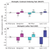
Binocular imbalance without lens/filter and under three lens/filter conditions. The bar graphs represent the mean interocular suppression ratio parameter at baseline and in the three conditions where the filter or lens is placed over either the left (OS) or right eye (OD). (A) Results from the DiCOT. (B) Results from the DLT. Error bars represent the bootstrapped 95% CI of the mean. Individual participant data are shown for each bar with the cross symbols.

Figure 4.

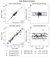
Test–retest reliability. The left column shows correlations between first and second (test and retest) measurements obtained using the DiCOT (A) and the DLT (C). The solid diagonal line indicates equality. Each point indicates a data point from one participant in one lens/filter condition (84 in total for the DiCOT, 82 in the DLT due to cases where a measurement result could not be obtained). The right column shows Bland–Altman plots giving the test–retest difference as a function of the mean of the two measures. The Bland–Altman plot for the DiCOT is given in B, corresponding to the test-retest plot in A. The Bland–Altman plot for the DLT is given in D, corresponding to the test-retest plot in C. The three black lines show the bias and the upper and lower LoA. The shaded region around each line gives the 95% CI. The results for each filter or lens condition are shown individually in Figure A1, and the statistics are reported in Table 1.

Figure 5.

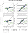
Comparison between DLT and DiCOT. The left column shows scatterplots comparing the measurement made with one test against that made with the other. The top row (A) compares the test (first) measurements, and the bottom (C) compares the second (retest) measurements. The diagonal green line is the best-fitting linear relationship (parameters given in green text). The black line shows equality. The right column shows Bland–Altman plots derived from the scatterplots (B for the first measurements, D for the second measurements). The three black lines show the bias and the upper and lower LoA. The shaded region around each line gives the 95% CI. The diagonal green line is the best-fitting linear relationship (parameters given in green text). The results for each filter or lens condition are shown individually in Figure A2, with statistics reported in part in Table 2 and in full in Table A1.

Figure 6.

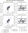
Comparison between DLT and adjusted DiCOT measurements. Panel A shows the relationship between the two measurements for the first (test) measurements, with the Bland–Altman plot shown in B. Panel C shows the relationship for the second (retest) measurements with the Bland–Altman plot shown in D. Similar to Figure 5; however, in this case the DiCOT values are adjusted according to the best-fitting linear relationships shown in green in Figure 5A (for the test measurements) and Figure 5C (for the retest measurements). The results for each filter or lens condition are shown individually in Figure A3, with statistics reported in-part in Table 2 and in-full in Table A2.

Figure A1.

Test–retest reliability. The data of Figure 4 are replotted here, separated into the different filter or lens conditions (rows). The first two columns show the DiCOT measurements. The remaining two columns show data from the DLT. In each pair, the left column shows correlations between test and retest measurements. The solid diagonal line indicates equality. Each point indicates a data point from one participant in one lens/filter condition. The right column shows Bland–Altman plots giving the test–retest difference as a function of the mean of the two measures. The three black lines show the bias and the upper and lower LoA. The shaded region around each line gives the 95% CI.

Figure A2.

Comparison between DLT and DiCOT. The data of Figure 5 are replotted here, separated into the different filter or lens conditions (rows). The first two columns show comparisons of the test (first) measurements. The remaining two columns show comparisons of the retest (second) measurements. In each pair, the left column shows scatterplots comparing the measurement made with one test against that made with the other. The diagonal green line is the best-fitting linear relationship (parameters given in green text). The black line shows equality. The right column shows Bland–Altman plots derived from the scatterplots. The three black lines show the bias and the upper and lower LoA. The shaded region around each line gives the 95% CI. The diagonal green line is the best-fitting linear relationship (parameters given in green text).

Figure A3.

Comparison between DLT and adjusted DiCOT measurements. Similar to Figure A2, but with DiCOT values adjusted according to the linear relationships reported in Figure A2.

References

1. Alais, D. (2012). Binocular rivalry: Competition and inhibition in visual perception. Wiley Interdisciplinary Reviews: Cognitive Science, 3, 87–103, 10.1002/wcs.151. - DOI - PubMed
1. Angelucci, A., & Shushruth, S. (2013). Beyond the classical receptive field: Surround modulation in primary visual cortex. In: Werner J. S. & Chalupa L. M. (Eds.), The new visual neurosciences, (pp. 425–444). Cambridge, MA: MIT Press.
1. Arnold, D. H., Grove, P. M., & Wallis, T. S. A. (2007). Staying focused: A functional account of perceptual suppression during binocular rivalry. Journal of Vision, 7(7):7, 1–8, 10.1167/7.7.7. - DOI - PubMed
1. Ashraf, M., Mantiuk, R., Martinovic, J., & Wuerger, S. (2022). Suprathreshold contrast matching between different luminance levels. In: 30th Color and Imaging Conference Final Program and Proceedings: Color Science and Engineering Systems, Technologies, and Applications (pp. 219–224). Springfield, VA: Society for Imaging Science and Technology.
1. Babu, R. J., Clavagnier, S. R., Bobier, W., Thompson, B., & Hess, R. F. (2013). The regional extent of suppression: Strabismics versus nonstrabismics. Investigative Ophthalmology & Visual Science, 54, 6585, 10.1167/iovs.12-11314. - DOI - PubMed
LinkOut - more resources