Theta phase precession supports memory formation and retrieval of naturalistic experience in humans

Abstract

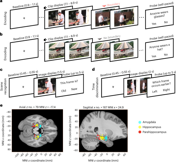
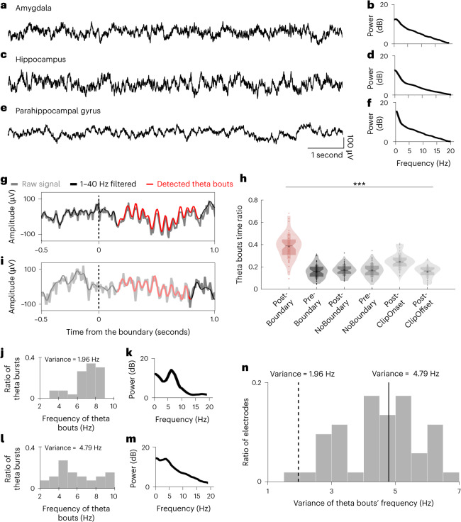
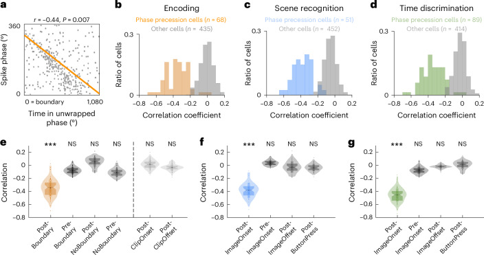
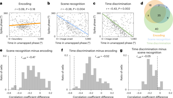
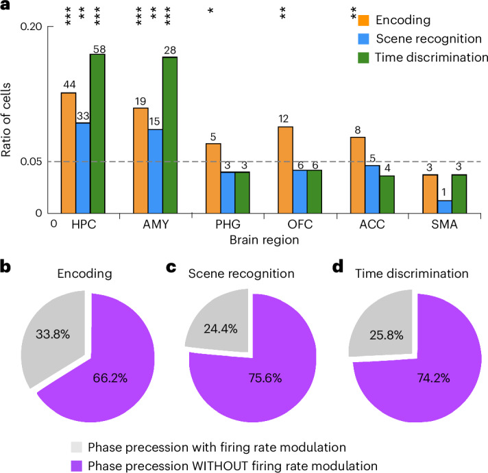
Associating different aspects of experience with discrete events is critical for human memory. A potential mechanism for linking memory components is phase precession, during which neurons fire progressively earlier in time relative to theta oscillations. However, no direct link between phase precession and memory has been established. Here we recorded single-neuron activity and local field potentials in the human medial temporal lobe while participants (n = 22) encoded and retrieved memories of movie clips. Bouts of theta and phase precession occurred following cognitive boundaries during movie watching and following stimulus onsets during memory retrieval. Phase precession was dynamic, with different neurons exhibiting precession in different task periods. Phase precession strength provided information about memory encoding and retrieval success that was complementary with firing rates. These data provide direct neural evidence for a functional role of phase precession in human episodic memory.

Fig. 1. Experiment and electrode locations.

a–d, Schematics of the three task stages. During encoding (a,b), the participants watched a series of silent clips and were instructed to answer yes/no questions that appeared randomly after every four to eight clips. These clips contained either cuts to scenes from the same or a different movie (a, boundary clips) or no cuts (b, no-boundary clips). The red triangle in a marks the time point of the boundary in an example boundary clip. The grey triangle in b indicates the time point of four seconds in an example no-boundary clip. During scene recognition (c), the participants were presented with a static image and were asked to indicate whether the image was ‘old’ (shown in the watched clips) or ‘new’. During time discrimination (d), the participants were presented with two images side by side and were asked to indicate whether the left or right frame appeared first in the watched clips. See ref. for more detailed information about the task. Due to copyright restrictions, the example images shown here are not the original stimuli used in the experiments. All images were generated by the authors. e, Locations of the 50 microelectrodes in the MTL across 22 participants (see the participants’ demographics in Supplementary Table 1) that had phase precession neurons. Shown is a slice from the template brain CIT168 (Methods), with microelectrodes plotted as individual dots and colour-coded for different brain regions (cyan for the amygdala, yellow for the hippocampus and red for the parahippocampal gyrus). The MNI coordinates for all microelectrodes in the plot are listed in Supplementary Table 2.

Fig. 2. Characteristics of theta bouts during encoding.

a–f, Example LFPs recorded from microelectrodes located in the amygdala (a), hippocampus (c), and parahippocampal gyrus (e). Panels b,d,f show LFP power spectra from the same example electrodes in a,c,e recorded throughout the entire task. g,i, Examples of detected theta bouts. The raw LFP (grey), 1–40 Hz band-pass-filtered LFP (black) and detected theta bout (red) are shown. t = 0 is the time point when a boundary occurs. h, Proportion of time occupied by theta bouts within different one-second time windows (analysis windows) before (Pre-Boundary) and after boundaries (Post-Boundary) in boundary clips, before (Pre-NoBoundary) and after (Post-NoBoundary) the midpoint in no-boundary clips, and after clip onsets (Post-ClipOnset) and clip offsets (Post-ClipOffset) of all the clips. Each dot represents one microelectrode (n = 50 in total). The asterisk and horizontal line denote the mean and median of the data, respectively. The shaded violin shape represents the data distribution, with the lower end indicating the 1st percentile (minima) and the top end indicating the 99th percentile (maxima). The top edge and bottom edge of the shaded rectangle represent the mean + s.d. and mean − s.d., respectively. The top edge and bottom edge of the shaded hourglass represent the 75th and 25th percentiles, respectively. ***P = 6 × 10⁻⁷ (two-tailed ANOVA test across all the analysis windows). j,l, Frequency of all detected theta bouts within the Post-Boundary time windows for the two example microelectrodes shown in g and i, respectively. The variance is also shown. k,m, Power spectra of the LFPs across all the Post-Boundary windows from the microelectrodes in g and i, respectively. n, Variance of the frequency of theta bouts across all recorded microwires in the MTL. The dashed and solid lines mark the variance of the two example microelectrodes shown in g and i, respectively.

Fig. 3. Prevalence of theta phase precession across different task stages.

a, Example hippocampal phase precession neuron during encoding. The spiking phases relative to local theta (y axis) are plotted as a function of time in unwrapped theta phase (Methods). Each dot shows one spike within three theta cycles (x axis) relative to boundaries. The orange line indicates the fitted correlation between neuronal spiking phase and time in unwrapped theta phase. b–d, Distribution of correlation coefficients for all MTL neurons demonstrating phase precession during encoding (b, orange), scene recognition (c, blue) or time discrimination (d, green). The distribution of correlation coefficients for neurons without phase precession is plotted in grey. Note that strong phase precession is indicated by negative correlation coefficients. e, Comparison of phase precession strength during encoding for the phase precession neurons in b (n = 68). Plotted are circular–linear correlation coefficients computed using spikes within three theta cycles before (Pre-Boundary) and after (Post-Boundary) boundaries, after clip onsets (Post-ClipOnset) and after clip offsets (Post-ClipOffset) in boundary clips, as well as before (Pre-NoBoundary) and after (Post-NoBoundary) the midpoint in no-boundary clips. ***P = 4 × 10⁻⁵ (two-tailed t-test against zero); NS, not significant. f,g, Comparison of phase precession strength during scene recognition (f) or time discrimination (g) for the phase precession neurons in c (n = 51) and d (n = 89), respectively. Plotted are circular–linear correlation coefficients computed using spikes within three theta cycles before (Pre-ImageOnset) and after image onsets (Post-ImageOnset), after image offsets (Post-ImageOffset) and after making a memory choice (Post-ButtonPress). The asterisk and horizontal line denote the mean and median of the data, respectively. The shaded violin shape represents the data distribution, with the lower end indicating the 1st percentile (minima) and the top end indicating the 99th percentile (maxima). The top edge and bottom edge of the shaded rectangle represent the mean ± s.d. and mean − s.d., respectively. The top edge and bottom edge of the shaded hourglass represent the 75th and 25th percentiles, respectively. ***P = 3 × 10⁻⁸ in f and ***P = 7 × 10⁻⁸ in g, two-tailed t-test against zero.

Fig. 4. Comparison of phase precession strength across different task stages.

a–c, Example hippocampal neuron whose spiking exhibited phase precession during scene recognition and time discrimination, but not encoding. Shown are spike phases as a function of time in unwrapped theta phase, displayed separately for encoding (a; t = 0 is the boundary in boundary clips), scene recognition (b; t = 0 is the image onset) and time discrimination (c; t = 0 is the image onset). The coloured lines indicate the fitted correlation between spike phase and time in unwrapped theta phase. The correlation value and its statistical significance (two-tailed permutation test) are listed above each plot. d, Number of MTL neurons showing significant phase precession during encoding (orange), scene recognition (blue), time discrimination (green) and combinations thereof. e, Difference in phase precession strength between encoding and scene recognition for neurons that show phase precession for encoding and/or scene recognition (that is, the orange plus blue circles in d). f, Difference in phase precession strength between encoding and time discrimination for neurons that showed significant phase precession during encoding and/or time discrimination (that is, the orange plus green circles in d). g, Difference in phase precession strength between scene recognition and time discrimination for neurons that showed significant phase precession during recognition and/or time discrimination (that is, the blue plus green circles in d). Note that in e–g, more negative correlations indicate stronger phase precession. The dashed lines indicate the example hippocampal neuron shown in a–c.

Fig. 5. Anatomical distribution of phase precession neurons and their co-occurrence with firing rate changes.

a, Phase precession was most prominent in the MTL. The bars indicate the proportion of neurons that exhibited phase precession in each anatomical area during different task stages (orange for encoding, blue for scene recognition and green for time discrimination). The number of phase precession neurons in each anatomical area is listed at the top of each bar. The dashed horizontal line indicates the chance level. The asterisks mark brain areas under specific task stages with proportions of phase precession neurons larger than expected by chance (P < 0.05, one-tailed binomial test). HPC, hippocampus; AMY, amygdala; PHG, parahippocampal gyrus; OFC, orbitofrontal cortex; ACC, anterior cingulate; SMA, supplementary motor area. b, Most phase precession neurons did not exhibit modulation by firing rate. Shown are the proportions of phase precession neurons in the MTL with and without firing rate modulation (defined as firing rate differences between before and after boundaries during encoding). c,d, Same as b but assessing whether neurons changed their firing rate between before and after image onset during scene recognition (c) or time discrimination (d). ***P < 0.001; **P < 0.01; *P < 0.05.

Fig. 6. Strength of phase precession is predictive of memory encoding and retrieval success.

a, Model comparisons for neural activity during the scene recognition task. Each bar shows a comparison between the full GLM model and reduced GLM models with or without (w/wo) a given predictor. A likelihood ratio bigger than 1 with a significant P value indicates a better model performance in explaining participants’ behaviour outcomes with the added predictor. The predictors considered are firing rate during encoding (Fr_encoding) and scene recognition (Fr_sceneRecog), and phase precession strength during encoding (r_encoding) and scene recognition (r_sceneRecog). b, Same as a, but for the time discrimination task. The predictors considered are firing rate during encoding (Fr_encoding) and time discrimination (Fr_timeDiscrim), and phase precession strength during encoding (r_encoding) and time discrimination (r_timeDiscrim). All the models in a and b consider all the recorded neurons in the MTL. c,d, Odds ratios for different predictors when predicting participants’ memory performance during scene recognition (c) and time discrimination (d). The vertical lines indicate the confidence intervals. The horizontal dashed line marks the chance level. The asterisks denote significance. e, For the winning model for scene recognition (indicated by the red box in a), the proportion of variance in the response variable (correct versus incorrect) explained by different groups of neurons is shown. Shown are R² ratios of models built using all phase precession neurons during encoding (orange line), all phase precession neurons during scene recognition (blue line) and all non-phase-precession neurons (grey bars). The total numbers of neurons used for the GLM model for each group were balanced by random subsampling. To do so, the non-phase-precession neuron group was subsampled 100 times, each time selecting the same number of neurons as the number of phase precession neurons present during scene recognition. The dashed line indicates the chance level. f, Same as e, but for time discrimination. Shown is the proportion of variance in the behaviour explained by the winning model (indicated by the red box in b). Shown are model fit for all phase precession neurons selected during encoding (orange), all phase precession neurons selected during time discrimination (green) and all other neurons (grey, subsampled 100 times and each time with the same number of neurons as those selected during encoding). The dashed line indicates the chance level. *P < 0.05; **P < 0.01; ***P < 0.001 in a–d.

Extended Data Fig. 1. Comparison of theta bout properties between task stages.

(a-c) Power spectra of local field potentials recorded during scene recognition averaged across all microelectrodes and the entire task within the indicated brain area. The shaded area indicates the standard error mean. (e-g) Same, but for time discrimination. (d and h) Proportion of the 1 s long analysis window occupied by theta bouts detected in microelectrodes (n = 50) during following the onset of image, baseline, and probe (decision) during scene recognition (d, **p = 2 × 10⁻³, two-tailed ANOVA test) and time discrimination (h, **p = 2 × 10⁻³, two-tailed ANOVA test). (i) Proportion of time that theta bouts detected in microelectrodes (n = 50) occupy 0 to 1-second after cognitive boundaries (encoding) or after image display (sceneRecog and timeDiscrim). Encoding vs scene recognition: **p = 0.002, encoding vs time discrimination: ** p = 0.007, scene recognition vs time discrimination: n.s. = not significant, Kolmogorov-Smirnov test. (j) Comparison of the variance of frequency for theta bouts detected in microelectrodes (n = 50) within the 0 to 1-second after cognitive boundaries (encoding) or after image display (sceneRecog and timeDiscrim). Encoding vs scene recognition: *p = 0.021, encoding vs time discrimination: ** p = 0.022, scene recognition vs time discrimination: n.s. = not significant, Kolmogorov-Smirnov test.

Extended Data Fig. 2. Characteristics of the local field potential signal.

(a and b) Time frequency plots of all the theta bouts (a) or theta bouts following boundaries (b) that are detected from a representative microelectrode with phase precession neurons identified. Time zero refers to the onset of theta bouts. (c-e) Time frequency plots of local field potential signals recorded from the same microelectrode shown in (a and b), aligned to boundaries (c), clip onsets (d), and clip offsets (e). (f) Frequency difference between cycles (1 vs 2, 2 vs 3, 1 vs 3) where all the theta bouts detected from the microelectrodes (n = 50) that phase precession neurons are identified. (g and h) Comparison of averaged theta power (g) and theta frequency (h) computed from local field potential signals within three theta cycles following boundaries, clip onsets and clip offsets in all microelectrodes with phase precession neurons identified (n = 50). **p = 3 × 10⁻³, n.s. = not significant (p > 0.05) in (g and h) for two-tailed ANOVA test.

Extended Data Fig. 3. Relationship between phase resetting and phase precession.

(a) Lower panel: theta phases from the local field potential signal recorded in a microelectrode where a phase precession neuron was identified. Upper panel: the inter-trial phase coherence (ITPC) was computed across all the trials from this microelectrode and was plotted as a function of time. Grey shaded area indicates significantly consistent phase coherence across trials, or phase resetting. (b) Averaged ITPC computed within 500 ms time window following soft boundaries versus hard boundaries separately for all the microelectrodes where a phase precession neuron was identified (n = 50). The asterisk and horizontal line denote the mean and median of the data, respectively. The shaded violin shape represents the data distribution with lower end of 1^st percentile (minima) and top end of 99^th percentile (maxima). The top edge and bottom edge of the shaded rectangle represent the mean ± std. and mean – std., respectively. The top edge and bottom edge of the shaded hourglass represents the 75^th and 25^th percentile, respectively. **p = 0.006 (two-tailed ANOVA test). (c) Ratio of phase precession neuron showing significant phase precession following only soft boundaries (SB), only hard boundaries (HB) or both conditions. (d) Correlation between ITPC and the time ratio of theta bouts occupied within the phase precession analysis windows (Pearson’s correlation). Each dot represents one microelectrode with phase precession neurons detected. (e-g) Among all the microelectrodes with phase precession neurons detected during encoding (c), scene recognition (d), and time discrimination (e), the proportion of channels showing theta phase resetting (dark blue) or not (light blue).

Extended Data Fig. 4. Neurons that exhibit theta-band phase locking and/or phase precession.

(a) The distribution of spiking phases during the entire task from an example phase locking neuron recorded in the hippocampus. (b-d) Proportion of neurons that demonstrate phase locking only (blue), transient phase precession only (green), both phase locking and transient phase precession (yellow), and none (brown) during encoding (b), scene recognition (c), or time discrimination (d).

Extended Data Fig. 5. Relationship between preferred phase changes in phase locking and phase precession.

(a-b) Example neuron. The distribution of spiking phase (relative to theta) of a phase precession neuron recorded within 1-second time window before (a) and after (b) boundaries is shown Significance level was assessed using the permutation test. (c) Proportion of phase precession neurons that demonstrate phase locking only within the 1-second time window before boundaries/image presentation, only within the 1-second time window after boundaries/image presentation, during both time windows but with different phases (that is, phase locking shifts), or no phase locking during either time windows.

Extended Data Fig. 6. Relationship between theta bouts and phase precession.

(a-b) Example neuron. Shown are the spike phases of spikes following boundaries plotted separately for trials (balanced trial numbers) with (a) or without theta bouts detected (b). Phase precession was observed in either case Significance was accessed using the permutation test. (c-e) Among all the phase precession neurons, their phase precession strength (that is, correlation coefficient) computed separately for trials with and without theta bouts detected during encoding (c), scene recognition (d), and time discrimination (e). **p = 5 × 10⁻³, *p = 0.032, n.s. = not significant, two-tailed paired t-test.

Extended Data Fig. 7. Phase precession quantified using method 1 and 2.

(a-d) Calculation for Method 1. Two example hippocampal neurons’ (recorded on the microelectrodes shown in Fig. 2g and i). Spike phases (relative to theta oscillations) are plotted as a function of time in seconds (a and c) or time in unwrapped theta phases (b and d), aligned to boundaries. Phase precession is quantified as the circular-linear correlations between neuronal spiking phases and time in seconds (a and c) or time in unwrapped theta phases (b and d). Pink lines indicate the correlation, with the correlation value and its statistical significance listed on the top of each subplot. (e-h) Further calculations for Method 2. The spike-time autocorrelation (e and g) and spike-phase autocorrelation (f and h) plots for the same neurons in (a-d). Blue lines indicate the decaying sine wave function fitted to the autocorrelation plots. Inset show the spike-phase spectra, with power as the y-axis and the relative frequency between the frequency of spiking and frequency of theta oscillations as the x-axis. Phase precession is quantified using the modulation index (MI), which is defined as the fraction between the peak height divided by the area under the curve in the spike-phase spectra plot. The modulation index and its statistical significance are listed on the top of each subplot. (i and j) Correlation coefficients (i) and modulation indices (j) for significant (pink) versus non-significant (gray) phase precession neurons as identified using Method 1 and Method 2, respectively. (k-l) Comparison of phase precession strength estimated using time in seconds and time in unwrapped phase for both method 1 and 2. (k) Differences in correlation coefficients as estimated using Method 1 (for example, |r in b – r in a|) against the frequency variance of theta bouts detected in these microelectrodes for significant neurons during encoding. (l) Differences in phase precession strength estimated with Method 2. Plotted is the difference in the modulation index (l, for example, |MI in f – MI in e|) against the frequency variance of theta bouts detected in these microelectrodes for significant neurons during encoding. In k and l, each dot represents one neuron. The empty circle represents the two example neurons in (a-h). Color lines indicate the fitted linear regression, with the correlation value and its statistical significance listed on the top of each plot. Significance was assessed using the permutation test in (a-h) and Pearson’s correlation in (k-l), respectively.

Extended Data Fig. 8. Comparison of phase precession when recognizing target (old) versus foil (new) images.

An example MTL neuron showing phase precession when the participant is asked to recognize target images (a) and foil images (b). Note that no significant phase precession is observed when identifying foil images. (c) Comparison between phase precession strength (correlation coefficient values) when participants are instructed to recognize target (blue) versus foil images (gray) across all phase precession neurons identified during scene recognition (n = 51). Each dot represents one neuron. The asterisk and horizontal line denote the mean and median of the data, respectively. The shaded violin shape represents the data distribution with lower end of 1^st percentile (minima) and top end of 99^th percentile (maxima). The top edge and bottom edge of the shaded rectangle represent the mean ± std. and mean – std., respectively. The top edge and bottom edge of the shaded hourglass represents the 75^th and 25^th percentile, respectively. Significance was assessed using the permutation test in (a, b) and two-tailed ANOVA test in (c, **p = 0.004), respectively.

Extended Data Fig. 9. Phase precession can exist without firing rate modulation.

Simulation based on the model of Mehta et al, 2002. (a and c) The spikes in this model (green dots) occur when the down-swing of the fluctuating inhibitory current (red) crosses the excitatory current (blue). Like in the original implementation, in this simulation neurons fired only briefly when excitation first exceeds inhibition. We implemented this feature by assuming a refractory period of 60 ms. Note that in both cases the firing rate of the neuron remains the same (number of spikes = 6). The difference is that the activation current is constant current in (a) and ramping in (d), resulting in no phase precession (b) and phase precession (d), respectively.

Extended Data Fig. 10. Comparison of phase precession strength between trials associated with correct versus incorrect memory performance.

(a-c) Phase precession during encoding grouped by recognition memory performance. An example MTL neuron showing phase precession following boundaries during encoding for trials that were later correctly recognized (a) but not for forgotten (incorrect) trials (b). (c) Comparison between phase precession strength (correlation coefficient values) between trials with correct (red) versus incorrect (grey) subsequent recognition memory across all phase precession neurons identified during encoding (n = 68). **p = 0.006 (d-f) Phase precession during encoding grouped by order memory performance. An example MTL neuron showing phase precession following boundaries during encoding for trials that were subsequently retrieved correctly (d) or incorrectly (e). (f) Comparison between phase precession strength (correlation coefficient values) between trials with correct (red) versus incorrect (grey) subsequent order memory across all phase precession neurons identified during encoding (n = 68). *p = 0.041. (g-i) Phase precession during scene recognition grouped by recognition memory performance. An example MTL neuron showing phase precession following image onsets when participant successfully (g) recognized tested images but no phase precession for incorrect trials (h). Note that, at group level, across all phase precession neurons identified during scene recognition (n = 51), their phase precession strengths do not show significant difference for trials with correct (red) versus incorrect (grey) subsequent recognition memory. n.s. = not significant. (j-l) Phase precession during time discrimination grouped by time discrimination performance. An example MTL neuron showing phase precession following image onsets when the participant successfully (j) retrieved the correct temporal order of tested images pairs but no phase precession for incorrect ones (k). (l) Comparison between phase precession strength between trials with correct (red) versus incorrect (grey) subsequent order memory across all phase precession neurons identified during time discrimination (n = 89). ***p = 8 × 10⁻⁴. Each dot represents one neuron. The asterisk and horizontal line denote the mean and median of the data, respectively. The shaded violin shape represents the data distribution with lower end of 1^st percentile (minima) and top end of 99^th percentile (maxima). The top edge and bottom edge of the shaded rectangle represent the mean ± std. and mean – std., respectively. The top edge and bottom edge of the shaded hourglass represents the 75^th and 25^th percentile, respectively. Significance was assessed using the permutation test in (a-b, d-e, g-h, j-k) and two-tailed ANOVA test in (c, f, i, l), respectively.

References

1. Lisman, J. E. & Jensen, O. The theta-gamma neural code. Neuron77, 1002–1016 (2013). - PMC - PubMed
1. Lisman, J. E. & Idiart, M. A. Storage of 7 ± 2 short-term memories in oscillatory subcycles. Science267, 1512–1515 (1995). - PubMed
1. Hopfield, J. J. Pattern recognition computation using action potential timing for stimulus representation. Nature376, 33–36 (1995). - PubMed
1. Bi, G. & Poo, M. Synaptic modification by correlated activity: Hebb’s postulate revisited. Annu. Rev. Neurosci.24, 139–166 (2001). - PubMed
1. Jensen, O. & Lisman, J. E. Position reconstruction from an ensemble of hippocampal place cells: contribution of theta phase coding. J. Neurophysiol.83, 2602–2609 (2000). - PubMed