Spiking representation learning for associative memories

Abstract

Networks of interconnected neurons communicating through spiking signals offer the bedrock of neural computations. Our brain's spiking neural networks have the computational capacity to achieve complex pattern recognition and cognitive functions effortlessly. However, solving real-world problems with artificial spiking neural networks (SNNs) has proved to be difficult for a variety of reasons. Crucially, scaling SNNs to large networks and processing large-scale real-world datasets have been challenging, especially when compared to their non-spiking deep learning counterparts. The critical operation that is needed of SNNs is the ability to learn distributed representations from data and use these representations for perceptual, cognitive and memory operations. In this work, we introduce a novel SNN that performs unsupervised representation learning and associative memory operations leveraging Hebbian synaptic and activity-dependent structural plasticity coupled with neuron-units modelled as Poisson spike generators with sparse firing (~1 Hz mean and ~100 Hz maximum firing rate). Crucially, the architecture of our model derives from the neocortical columnar organization and combines feedforward projections for learning hidden representations and recurrent projections for forming associative memories. We evaluated the model on properties relevant for attractor-based associative memories such as pattern completion, perceptual rivalry, distortion resistance, and prototype extraction.

Keywords: BCPNN; Hebbian learning; associative memory; attractor dynamics; representation learning; spiking neural networks; structural plasticity; unsupervised learning.

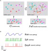
Figure 1

Conceptual schematic of functional roles of the different architectures and neuron-unit activation types investigated in this work. (A) In the feedforward-only network (Ff), the representations in the input space are highly correlated and data from distinct categories and with different features are entangled in complex non-linear relationships (shown as purple triangles, red star, and blue squares). The feedforward projections learn to map these data into the hidden space where the data points are less correlated and grouped together based on the feature similarity making them more linearly separable. The Full architecture that includes the recurrent projection utilizes the uncorrelated nature of the representations in the hidden space to form effective associative memories and group similar data points into attractors (attractor boundaries or basins of attraction shown as dashed circles and attractor states as symbol with golden border). (B) The activation function denoting the signal computed and communicated by each neuron-unit can be one of either Rate (non-spiking), Spk (spiking), or Spspk (sparsely spiking). The rate-based activation codes for the probability of the presence of a feature that the neuron-unit represents (“confidence”) and takes continuous values in the interval [0, 1]. The Spk activation is generated as stochastic binary samples from the underlying firing rate which can reach biologically implausible levels up to 1,000 Hz. The Spspk activation is generated as stochastic binary samples, but with firing rate scaled down to biologically realistic values with the maximum of 100 Hz.

Figure 2

Schematic of the network architecture. The input (INP), hidden (HID), and input reconstruction (INPRC) populations follow the columnar/modular architecture, i.e., they are modularized into hypercolumns, which in turn constitute minicolumn units locally competing through softmax normalization. The feedforward projections connect the INP with the HID populations, recurrent projections connect the HID units with other HID units, and the feedback projections connect the HID population with the INP population.

Figure 3

MNIST dataset modified for pattern completion, perceptual rivalry, and distortion resistance tasks sorted by difficulty level (column-wise) and type of modification (row-wise). (A) Pattern completion: the images are partially visible as a gray bar of varying width is placed on either the top, bottom, left, or right of image. (B) Perceptual rivalry: the images are partially overlapped with varying width by a randomly chosen rival image. (C) Distortion resistance: the images are modified by adding random flips (noise), regularly spaced grid lines (grid), randomly spaced black lines (clutter), randomly spaced white lines (deletion), or a grey square box (occlusion) with varying degree controlled by the difficulty level.

Figure 4

Protocol for network simulation. The network is run either in training mode (top row), where the feedforward-driven activities are used for synaptic learning and structural plasticity, or in evaluation mode (bottom row), where the feedforward-driven activities are used to cue the recurrence-driven associative memories. For each pattern, the network is run either for two phases (no-input and ffwd) in the training mode or for four phases in the evaluation mode (no-input, ffwd, overlap, and recr). The gray arrows converging on the INP and INPRC populations indicate injecting the MNIST images as inputs to the respective populations. The white unfilled arrows indicate the presence of a projection in the network connecting two populations. Blue filling on the projection arrows indicates propagation of activities through the respective projections. Purple filling on the projection arrows indicate the projection undergoes synaptic and structural plasticity updates for each pattern. Arrow with both blue and purple filling indicates the projection is both propagating and learning. In the no-input phase, the network is run without any input to clear any previous activity. In the ffwd phase the network is driven with the external input to the INP and INPRC populations and the INP population drives HID population. In the overlap phase the HID population is driven both by the INP population and itself through recurrent projections. In the recr phase the input is cutoff, and the HID population is running solely through recurrent self-projections.

Figure 5

Spiking activity and firing rate for the INP (left), HID (center), and INPRC (right) populations. The first row shows the spike rasters for the first 10 minicolumns (arranged within 5 hypercolumns) for the INP and INPRC population and the first 400 minicolumns (arranged within 4 hypercolumns) for the HID population. The white bars correspond to the no-input period (100 ms) and the gray bars correspond to the pattern period (ff, overlap, and recr combined; 300 ms). The bottom row shows the firing rate of two selected minicolumns (indicated by blue and red spike trains in their respective population) computed by convolving the spike trains with a Gaussian kernel (σ² = 20 ms) demonstrating the minicolumns that spike with the maximum firing rate around 100 Hz.

Figure 6

Representational similarity. Pair-wise cosine similarity matrices for N = 10,000 MNIST test patterns sorted by their labels for INP (left), HID (middle) and INPRC (right) populations at T = 100 ms (feedforward-driven; upper row) and T = 300 ms (attractor-driven; lower row) representations. The orthogonality ratio, s_ortho, is displayed inside each plot. The INP population shows low orthogonality due to the large similarity values (0.6–0.8) both within- and between-classes. The HID population (T = 100 and 300 ms) shows high orthogonality due to low similarity values (0–0.2) between-class owing to the sparse distributed nature of representations. The orthogonality ratio also increases from feedforward-driven representations (T = 100 ms) to attractor representations (T = 300 ms). The input reconstruction population, INPRC, shows more orthogonality when compared to the corresponding INP similarities.

Figure 7

Time course of attractor representations for one pattern. The spikes and z-traces of INP and INPRC populations for one example pattern for T = 300 ms. The spike raster is highly noisy and sparse while the z-traces show a highly stable representation of digits. The INPRC population shows the initial reconstruction of feedforward-driven representations (T = 60–180 ms) and the attractor reconstructions (T = 150–300 ms) driven by the recurrent projections showing a stable convergence to the prototypical digit (corresponding to one of the class labels) even after the input is no longer fed into the network.

Figure 8

Receptive field formation for feedforward (left) and feedback (right) projections. Each column corresponds to connections between one randomly chosen hypercolumn of the HID population (column number corresponds to index of HID hypercolumn) and the INP population. Over the course of training the connections form spatially localized receptive fields in the image space.

Figure 9

Convergence of the structural plasticity algorithm for feedforward (left) and feedback (right) projections. The number of rewiring flip operations (top row) and $\tilde{M}$ score (normalized mutual information; bottom row) per rewiring step over the course of training (mean ± std. from n = 100 HID hypercolumns) shows convergence for both feedforward and feedback projections.

Figure 10

Impact of z-filtering on classification performance. Higher value of ${\tau }_z$ and ${\tau }_m$ implies longer filtering and setting the value to 1 ms (=$\mathrm{\Delta }t$) implies essentially no filtering. Longer $z$-filtering compensates for low firing rates in sparsely firing spiking networks. For high firing rate ($f_{max}$ > 200 Hz; top rows), the accuracy is high over a wide range of ${\tau }_z$ and ${\tau }_m$ values. For sparsely firing networks with biologically realistic firing rates ($f_{max}$< 200 Hz; bottom rows), the performance is sensitive to ${\tau }_z$, optimal in range of 10–50 ms, and resistant to ${\tau }_m$ values.

Figure 11

Prototype extraction. (A) Distribution of pair-wise similarities (S) of HID attractor representations (T = 300 ms) with a clear mode close to zero and only a smaller fraction of high values. (B) The relationship between similarity threshold, S_min, and the number of prototypes found by grouping attractor representations into unique prototypes. (C) The prototypes found for S_min = 0.01 (upper), 0.1 (middle), and 0.2 (right) by averaging the input reconstructions from the z-traces of the INPRC population.

Figure 12

Time course of attractor representations in the (A) pattern completion, (B) perceptual rivalry, and (C) distortion resistance tasks. The spikes and z-traces of INP and INPRC populations for one example pattern are shown for each task (T = 300 ms; similar to the setup in Figure 6). The INP population is driven by the spiking inputs from the corrupted image (T = 0–150 ms) with (A) top gray bar, (B) occluded partially by another rival image, and (C) randomly occurring black noise. The INPRC population shows the reconstructed image in the feedforward-driven phase (INPRC z-traces; T = 60–120 ms) is the similar to the corrupted image with traces of the top bar. In the recurrent-driven phase (T = 180–300 ms) the reconstructed image is a cleaned version of the pattern and settles on a prototypical digit representation stored in the associative memory.

Figure 13

Comparison of classification performance on associative memory tasks. The sparsely spiking models (SpspkFf, SpspkFull) perform very closely to the rate (RateFf, RateFull) and spiking (SpkFf, SpkFull) models in all cases. For low difficulty levels (<0.4), the full network models (RateFull, SpkFull, and SpspkFull) do not offer a clear advantage (sometimes performance slightly worse) compared to their corresponding feedforward-only models (RateFf, SpkFf, and SpspkFf) models. However, there is a clear trend of improvement for the full models compared to the feedforward-only models once the difficulty level is above 0.4 in all associative memory tasks. The error bars are standard deviation from n = 5 runs.

References

1. Amit D. J. (1989). Modeling brain function. The World of Attractor Neural Networks, Cambridge University Press: Cambridge University Press.
1. Amit D. J., Gutfreund H., Sompolinsky H. (1987). Information storage in neural networks with low levels of activity. Phys Rev A (Coll Park) 35:2293. doi: 10.1103/PhysRevA.35.2293 - DOI - PubMed
1. Anderson J. R., John R., Bower G. H., (1973). Human associative memory: A brief edition
1. Bailey C. H., Kandel E. R. (1993). Structural changes accompanying memory formation. Annu. Rev. Physiol. 55, 397–426. doi: 10.1146/annurev.ph.55.030193.002145 - DOI - PubMed
1. Bartlett F. C., Kintsch W., (1995). Remembering: A study in experimental and social psychology
LinkOut - more resources