Genetic architecture reconciles linkage and association studies of complex traits

Abstract

Linkage studies have successfully mapped loci underlying monogenic disorders, but mostly failed when applied to common diseases. Conversely, genome-wide association studies (GWASs) have identified replicable associations between thousands of SNPs and complex traits, yet capture less than half of the total heritability. In the present study we reconcile these two approaches by showing that linkage signals of height and body mass index (BMI) from 119,000 sibling pairs colocalize with GWAS-identified loci. Concordant with polygenicity, we observed the following: a genome-wide inflation of linkage test statistics; that GWAS results predict linkage signals; and that adjusting phenotypes for polygenic scores reduces linkage signals. Finally, we developed a method using recombination rate-stratified, identity-by-descent sharing between siblings to unbiasedly estimate heritability of height (0.76 ± 0.05) and BMI (0.55 ± 0.07). Our results imply that substantial heritability remains unaccounted for by GWAS-identified loci and this residual genetic variation is polygenic and enriched near these loci.

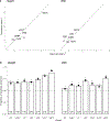
Extended data Figure 1.. Observed and theoretically predicted statistics for locus-specific linkage analysis.

Panel a, the observed and predicted mean test statistics of linkage (${\chi }^2$) test statistics for height and BMI. The error-bars indicate standard errors (s.e.) calculated as the standard deviation of locus-specific statistics divided by the square root of the effective number independent markers, that is ~$94$ (Supplementary Table 8). The size of the circle is proportional to sample size. The theoretically predicted values are based on the REML estimates of heritability from genome wide IBD regression (${\widehat{h}}_{FS}^2$) and the observed correlation between siblings. Panel b, the proportion of loci with positive (i) estimated linkage (the bars and the values) and (ii) theoretically predicted (the black rectangles +/- s.e., Methods). The dotted horizontal line represents the proportion (i.e., 0.5) expected in the absence of a genetic contribution to the trait. The data is shown for Generation Scotland (GS, number of quasi-independent sib-pairs (n) = 8,368), the Queensland Institute of Medical Research cohort (QIMR, n = 12,844), the Lifelines Cohort (LL, n = 16,581), the UK Biobank (UKB, n = 21,756), the Estonian Biobank (EBB, n = 25,333), the HUNT study (HUNT, n = 34,575) and the meta-analysis combining all cohorts (META, n = 119,457). The numerical values for mean and median ${\chi }^2$ and proportion of ${\chi }^2$ > 0 are presented in Supplementary Table 7A.

Extended data Figure 2.. Effect of polygenicity and sample size of linkage studies on the correlation between predicted and observed linkage signals in simulated data.

The results are shown for 8 simulated genetic architectures (polygenicity = 0.1%-100%) with a genome-wide $h^2=1$. a-b, show the observed and predicted linkage signals (measured as variance explained) on chromosomes 1 and 22, respectively, for one simulation replicate. The simulated causal variants are depicted as green stars. The predicted signal, estimated as a weighted sum of simulated effects (Methods, Eq. 1) is depicted by the black curve. The grey and yellow lines show the observed linkage signal from the analysis of 20,000 and 100,000 simulated sib-pairs, respectively, where the phenotypes were simulated using the same causal variants (green stars). The correlations $\widehat{\varphi }$ for each polygenicity panel are the chromosome-wide estimates for each linkage sample size (yellow: n=20,000; grey: n=100,000). c, the summary of results across 100 replicates. $\widehat{\varphi }$ is estimated per chromosome across the grid of 0.5 cM, then a chromosome length weighted average is calculated for each replicate. Each symbol represents a mean value across 100 simulation replicates and the error bars are standard deviation across replicates. The left-most enlarged symbols for each polygenicity panel indicate that the true simulated SNP effects were used predict linkage signal, i.e., the expected prediction accuracy from polygenic scores ($R_g^2$) using these causal variants = 1. To approximate estimation errors of SNP effects in a GWAS of finite sample, $\widehat{\varphi }$ was also calculated using causal variants with $R_g^2<1$ (regular symbols). For the numeric values see Supplementary Table 9. Estimated variance components were not constrained to ensure unbiasedness. Therefore, if a region of the genome does not explain any genetic variation, then 50% of the estimates are expected to be negative.

Extended data Figure 3.. Colocalization between GWAS-predicted and observed linkage signals for traits adjusted for polygenic scores (PGS).

Panel a, the correlation between observed linkage signals for PGS-adjusted height and predicted linkage signals from 12,010 height-associated SNPs. Panel b, the correlation between observed linkage signals for PGS-adjusted BMI and predicted linkage signals from 787 BMI-associated SNPs. Height was adjusted using a PGS based on the same 12,010 height-associated SNPs (explaining 38% of height variance), while BMI was adjusted using a PGS including 4,582 SNPs (explaining 9% of BMI variance). The x-axis in each panel displays the correlation ($\widehat{\varphi }$) between observed and predicted (from GWAS results; Methods) linkage signals. In each panel, the vertical dashed line represents the correlation between observed and predicted linkage signals from either height-associated SNPs (a) or 787 BMI-associated SNPs (b). Predicted linkage signals were also obtained under the null hypothesis (that is “the correlation between observed and predicted linkage signals is due to the curvature effect”) using 1,000 draws of random SNPs with similar minor allele frequency and linkage disequilibrium properties as trait-associated SNPs. The histogram in each panel represents the distribution of correlations (under the null) between observed linkage for the trait indicated in the corresponding column-panel and predicted linkage obtained from these 1,000 draws. The mean of correlations obtained under the null hypothesis is denoted ${\widehat{\varphi }}_{\mathrm{C}\mathrm{E}}$. The P-values (P) reported in the top-left corner of each panel assess the statistical significance of the difference between $\widehat{\varphi }$ and ${\widehat{\varphi }}_{\mathrm{C}\mathrm{E}}$ using a two-sided Wald test. Numeric values are presented in Supplementary Table 10.

Extended data Figure 4.. Correlation between chromosome length and estimates of variance explained from linkage analyses of BMI.

Analyses were based on summary statistics from a linkage meta-analysis of BMI and BMI adjusted for polygenic score (PGS). The x-axis represents the physical length of each chromosome relative to the size of the autosome (i.e., ~2879 Mb). The y-axis represents the expected variance explained ($q_{\mathrm{s}}^2$) for each chromosome ($s=1-22$) estimated as $q_{\mathrm{s}}^2={m_s\stackrel{-}{q}}^2$, where ${\stackrel{-}{q}}^2$ is the mean across the chromosome of estimates of locus-specific variance, and $m_s$ an effective number of independent markers per chromosome (Supplementary Table 8). Error bars around each dot represent $m_s$ times the standard deviation of linkage estimate across the chromosomes. Standard errors (s.e.) of the regression slopes were obtained using a leave-one-chromosome-out jackknife approach. 95% confidence intervals (CI) were calculated as 1.96$\times$s.e.

Figure 1.. Recombination-rate stratified estimates of heritability (hFS2)andproportionofvarianceduetocommonsiblingeffectsuncorrelatedwithIBDsharing(c2) for height (a) and BMI (b).

a–b, Estimates were obtained using restricted maximum likelihood in six cohorts of European-ancestry individuals: the UK Biobank (UKB), Generation Scotland (GS), the Lifelines Study (LL), the Queensland Institute of Medical Research cohort (QIMR), the Estonian Biobank (EBB), the HUNT study (HUNT) and the fixed-effect meta-analysis results combining all cohorts (META). The number of quasi-independent sib-pairs (n) for each trait and cohort is indicated on y-axis. Each dot represents a point estimate, and the corresponding error bar represents its standard error (s.e.). Numeric values are given in Supplementary Table 3. Estimated variance components were not constrained to be positive to ensure unbiasedness.

Figure 2.. Chromosomes containing loci significantly linked with height.

Linked loci were identified from the meta-analysis of 119,457 quasi-independent sibling-pairs before and after adjustment for genetic predictors (PGS, polygenic score) derived from the largest available GWAS of height (average proportion of height variance explained across cohorts: $R^2=0.38$). The genetic position of independent trait-associated SNPs is represented below the y=0 line by blue dots, which radius is proportional to the association ${\chi }^2$ statistic. Results for all the autosomes for height and BMI are shown in Supplementary Fig. 4a–b. The vertical dashed lines indicate the two LOD drop-off confidence interval (relative to the peak LOD score) on each side of a genetic position where the linkage LOD score exceed 3.6 (Table 1). The black horizontal dotted line represents the threshold for significantly linked loci (LOD score ≥ 3.6). The grey horizontal dashed line indicates a LOD score of 0.

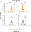
Figure 3.. Colocalization between observed and GWAS-predicted linkage signals.

Row-panels (row 1 = panel a and b; row 2 = panel c and d) represent predicted linkage signals based on a given set of trait-associated SNPs and column-panels represent observed linkage signals for height (panels a and c) and body mass index (BMI; panels b and d). The x-axis in each panel displays the correlation ($\widehat{\varphi }$) between observed and predicted (from GWAS results; Methods) linkage signals. The y-axis represents counts. In each panel, the vertical dashed line represents the correlation between observed linkage signals for the trait specified in the corresponding column-panel header and predicted linkage signals from either 12,010 height-associated SNPs (panels a and b) or 787 BMI-associated SNPs (panels c and d). Predicted linkage signals were also obtained under the null hypothesis (that is “the correlation between observed and predicted linkage signals is due to the curvature effect”) using 1,000 draws of random SNPs with similar minor allele frequency and linkage disequilibrium properties as trait-associated SNPs. The histogram in each panel represents the distribution of correlations (under the null) between observed linkage for the trait indicated in the corresponding column-panel and predicted linkage obtained from these 1,000 draws. The mean of correlations obtained under the null hypothesis is denoted ${\widehat{\varphi }}_{\mathrm{C}\mathrm{E}}$. The P-values (P) reported in the top-left corner of each panel assess the statistical significance of the difference between $\widehat{\varphi }$ and ${\widehat{\varphi }}_{\mathrm{C}\mathrm{E}}$ using a two-sided Wald test (conditional on $\widehat{\varphi }$) and based on the sampling variance of ${\widehat{\varphi }}_{\mathrm{C}\mathrm{E}}$ across replicates. At a significance threshold P<0.05, our results imply that linkage signals for height are predictable from height-associated SNPs (panel a), but not from BMI-associated SNPs (panel c), and that linkage signals for BMI are also predictable from BMI-associated SNPs (panel d), but not from height-associated SNPs (panel b). Numeric values are presented in Supplementary Table 10.

Figure 4.. Correlation between chromosome length and estimates of variance explained from linkage analyses of height.

Analyses were based on summary statistics from a linkage meta-analysis of height and height adjusted for polygenic score (PGS) in 119,457 quasi-independent sibling pairs. Each dot represents a chromosome. The x-axis represents the physical length of each chromosome relative to the size of the autosome (i.e., ~2879 Mb). The y-axis represents the expected variance explained ($q_{\mathrm{s}}^2$) for each chromosome ($s=1-22$) estimated as $q_{\mathrm{s}}^2={m_s\stackrel{-}{q}}^2$, where ${\stackrel{-}{q}}^2$ is the mean across the chromosome of estimates of locus-specific variance, and $m_s$ an effective number of independent markers per chromosome (Supplementary Table 8). Error bars around each dot represent $m_s$ times the standard deviation of linkage estimate across the chromosomes. Standard errors (s.e.) of the regression slopes were obtained using a leave-one-chromosome-out jackknife approach. 95% confidence intervals (CI) for the regression slopes were calculated as 1.96×s.e.

References

1. Polderman TJC et al. Meta-analysis of the heritability of human traits based on fifty years of twin studies. Nat Genet 47, 702–9 (2015). - PubMed
1. Risch N & Merikangas K The future of genetic studies of complex human diseases. Science 273, 1516–1517 (1996). - PubMed
1. Lynch M & Walsh B Genetics and Analysis of Quantitative Traits. (Sinauer Associates, Inc., Sunderland, MA, 1998).
1. Botstein D & Risch N Discovering genotypes underlying human phenotypes: past successes for mendelian disease, future approaches for complex disease. Nat Genet 33, 228–237 (2003). - PubMed
1. Hall JM et al. Linkage of early-onset familial breast cancer to chromosome 17q21. Science 250, 1684–1689 (1990). - PubMed
LinkOut - more resources