Neural substrates for saccadic modulation of visual representations in mouse superior colliculus

Abstract

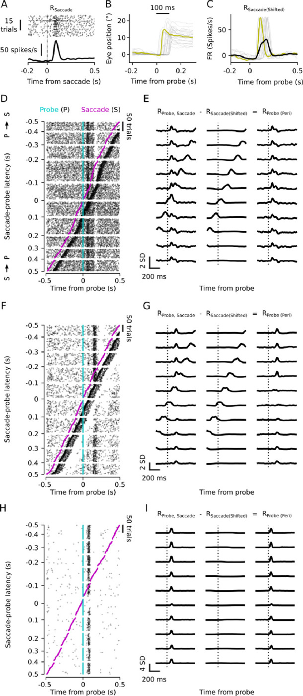
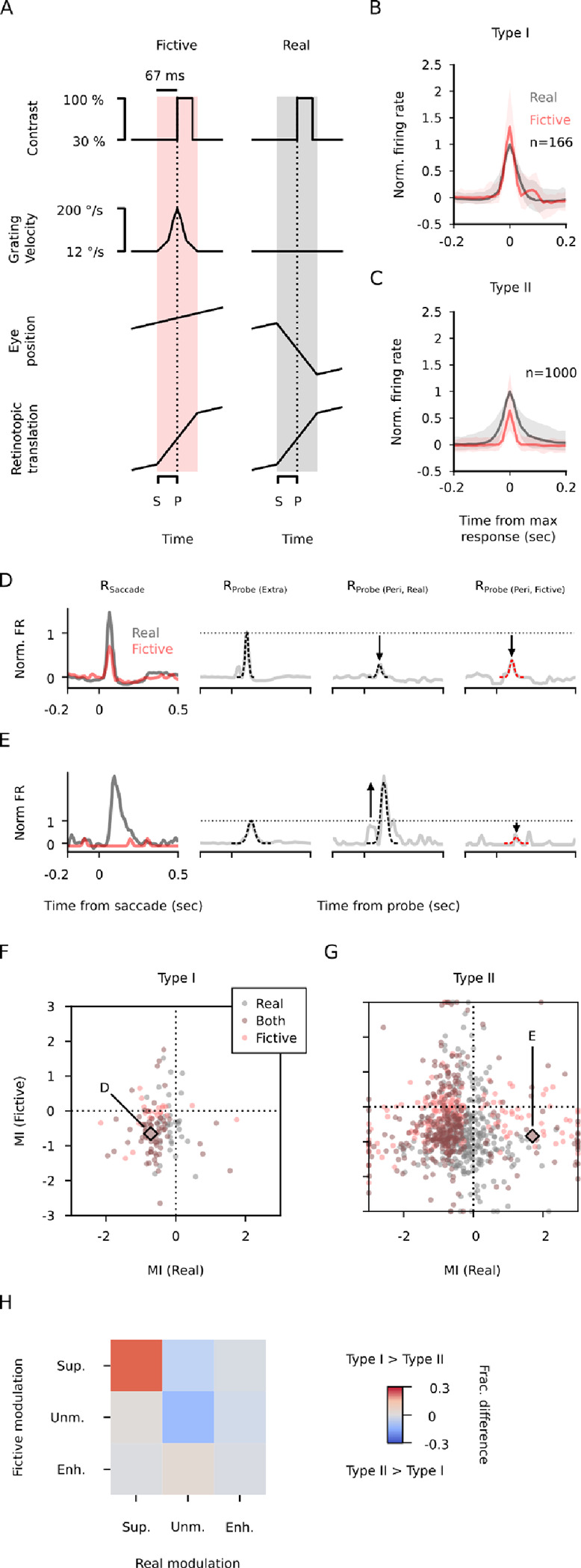
How do sensory systems account for stimuli generated by natural behavior? We addressed this question by examining how an ethologically relevant class of saccades modulates visual representations in the mouse superior colliculus (SC), a key region for sensorimotor integration. We quantified saccadic modulation by recording SC responses to visual probes presented at stochastic saccade-probe latencies. Saccades significantly impacted population representations of the probes, with early enhancement that began prior to saccades and pronounced suppression for several hundred milliseconds following saccades, independent of units' visual response properties or directional tuning. To determine the cause of saccadic modulation, we presented fictive saccades that simulated the visual experience during saccades without motor output. Some units exhibited similar modulation by fictive and real saccades, suggesting a sensory-driven origin of saccadic modulation, while others had dissimilar modulation, indicating a motor contribution. These findings advance our understanding of the neural basis of natural visual coding.

Figure 1.. Strategy for studying saccadic modulation.

A. Experimental design: head-fixed mice were presented with visual probes and drifting gratings to elicit saccades while cameras captured pupil positions and neuropixels probe recorded populations of visual SC units. B. Visual stimulus consisting of 90 s blocks of gratings drifting leftward or rightward with probes (0.05 s grating contrast increment) presented every 0.5–1 s. C. Distribution of peak eye movement velocity for leftward (orange) and rightward (blue) saccades or non-saccadic eye movements (black) across 47 sessions. Solid lines are means across sessions. Shaded region is mean ± 1 standard deviation. D. Distribution (mean ± 1 standard deviation) of S-P latencies for 44 sessions. Black barindicates −0.5 to 0.5 s perisaccadic window used for subsequent analyses. E. Coronal SC section showing electrode tract (DiO, green); red, Nissl. Scale bar, ~1000 μm. F. Receptive fields (RFs) for a subset of visual units from an example session, centered on eachunit’s center-of-mass position along the electrode. Color indicates azimuthal position of the RF centroid. G. All experimental time series (eye position, saccades, probes and spikes) for a ~15 s segmentof the example session, units are color coded by their RF position shown in F. Dotted lines indicate the appearance of the grating stimulus (left) and then the onset of grating motion (right).

Figure 2. SC visual units exhibit diverse neural representations of probes.

A. Raster (left) and trial-averaged, standardized peri-stimulus time histograms (PSTH; right) aligned to probe drifting in the preferred direction for an example unit with a positive, monophasic response. Left inset, ON (black) and OFF (gray) receptive fields. Right inset, individual components (shown in different colors) of the Gaussian mixtures model fit to the PSTH. Dashed line indicates the time of probe onset. B-D. Same as in A but for examples of biphasic, multiphasic and negative units, respectively. E. Amplitude-normalized PSTHs for all visual SC units used for subsequent analysis grouped by unit type. Arrows indicate examples in A-D.

Figure 3. Saccades modulate responses to probes.

A. Peri-saccade raster and trial-averaged firing rate (R_Sacccade) for an example unit (same example as in D-E). B. Eye position as a function of time relative to probe onset for trials in which the saccade occurred 0 to 100 ms following probe presentation. Representative saccade waveform is highlighted in yellow, corresponding to the latency-shifted trace of R_Saccade in C. C. S-P latency-shifted traces of R_Saccade corresponding to trials shown in B in which the saccade begins 0 to 100 ms following probe onset. R_{Saccade(Shifted)}, the average over all instances of R_Saccade, is shown in black. The yellow trace corresponds to the example saccade in B. D. Raster for a representative unmodulated unit with trials sorted by S-P latency from −500 ms to 500 ms in 100 ms bins. Black ticks, spikes; cyan, probe; magenta, saccade. Negative/positive S-P latencies specify probes preceding/following the saccade, respectively. E. Approach for isolating probe responses on trials with coincident saccades. Left column, R_Probe, Saccade; mean standardized firing rate for the observed perisaccadic response within each of the 100 ms time bins indicated in A. Middle column, R_{Saccade(Shifted)}; the estimated saccade-related activity in each bin, calculated as in C. Note that the shape of R_{Saccade(Shifted)} depends on recorded saccade occurrences (magenta in D) and thus is distinct for each time bin. Right column, R_Probe(Peri); the difference between R_{Probe, Saccade} and R_{Saccade(Shifted)}. The time of probe onset (cyan in D) is marked with a dashed vertical line. F-G. Same as in D-E, but for an example unit that exhibits a strong response to saccades and saccadic suppression. H-I. Similar to D-E, for an example unit that does not respond to saccades and exhibits saccadic suppression.

Figure 4. Saccadic suppression and enhancement exhibit distinct temporal dynamics.

A. R_Probe(Extra) and R_Probe(Peri), left and right, respectively, for an example unit that exhibits saccadic suppression (S-P latency=0 to 100 ms). Dashed lines, GMM component with the largest amplitude. B-C. Same as in A but for a unit that is not modulated (B) or is enhanced (C). D. Saccadic modulation for all visual SC units (n=1383) as a function of S-P latency. Units with significant suppression or enhancement (p<0.05, bootstrapping test) are indicated in blue or red, respectively. Black arrows, examples from A-C. E. Fraction of units suppressed (blue), enhanced (red), or unmodulated (gray) for each 100 msS-P latency bin. F. Neural trajectories representing the mean response to extrasaccadic probes (solid line) or perisaccadic probes (dashed line; S-P latency=0 to 100 ms) for an example population of simultaneously recorded visual SC units. G. Euclidean distance between extrasaccadic and perisaccadic population vectors for the example population shown in F. H. Fraction of sessions with a significant difference between extrasaccadic and perisaccadic population responses as a function of S-P latency.

Figure 5. Modulation peaks at specific time windows around the saccades.

A. Illustration of saccade-probe latency (S-P), probe-maximum response latency (P-M), and saccade-maximum response latency (S-M). B. Distribution of P-M latency for all visual SC units. C. Left, a family of R_Probe(Peri) responses for all S-P latency bins for an example unit with a short P-M latency. Right, R_Probe(Extra). Black arrow indicates R_Probe(Peri) with the lowest amplitude. Vertical and horizontal dotted lines indicate the time of saccade onset and the amplitude of R_Probe(Extra), respectively. Each individual R_Probe(Peri) shows the unit’s firing rate from 0 to 300 ms relative to probe presentation. D. Same as in C but for an example unit with a prolonged P-M latency. E. Top. Predicted pattern of suppression as a function of S-P and P-M latencies for three alternative hypotheses. Left, middle, and right cartoons indicate the pattern of suppression if suppression depends on S-P latency, P-M latency, or S-M latency, respectively. Lines to the left of the cartoons indicate the corresponding set of contours overlaid on the heatmap below. Bottom. Mean MI across all suppressed units (n=663) as a function of S-P latency (rows) and P-M latency (columns). Units on the left of the x-axis exhibit shorter P-M latencies whereas units on the right exhibit longer P-M latencies. This representation is constructed by first sorting the units based on their P-M latencies and assigning each unit to a single column. Then, the MI computed for each S-P latency is assigned to a row. Finally, the average MI is computed for each cell in this matrix. Dotted horizontal lines show expected contours if modulation depends only on S-P latency. Dashed vertical lines show expected contours if modulation depends only on P-M latency. Solid black lines show expected contours if modulation depends on S-M latency. White contours indicate mean MI < −0.35. F. Amplitude-weighted median MI for units exhibiting suppression but not enhancement for S-Platencies of −100 to 200 ms. Shading, interquartile range weighted by amplitude of R_Probe(Extra). Bottom bar shows latencies with median MI significantly different than zero (p<0.001, Wilcoxon signed-rank test). G. Same as in C but for a unit that exhibits enhancement. H. Same as in F but for units that exhibit enhancement during any S-P latency between −100 and 200 ms. I. The overlap of suppressed and enhanced units.

Figure 6. Saccadic modulation does not depend on directional tuning.

A. R_Probe(Extra) for probes in the preferred or null direction for an example direction-selective unit. B. Same as in A for an example unit that is not direction-selective. C. Distribution of horizontal direction-selectivity indices across units. Units with low signal-to-noise ratios (max(abs(R_{Probe(Extra, Pref.)})) < 0.5 SD) were excluded from this analysis. D. Fraction of units that are enhanced (red), unmodulated (gray), or suppressed (blue) as afunction of S-P latency for non-DS units (left) and DS units (right). E. Correlation between MI calculated for probes in the preferred and null directions, for non-DS and DS units.

Figure 7. Saccadic modulation arises from visual and non-visual mechanisms.

A. Schematic showing how fictive saccades (left) mimic the retinotopic translation of the probe (bottom) during real saccades (right). Saccade (S) and probe (P) times are indicated on the bottom. B. Median (±1 quartile) firing rate during real (gray) and fictive (red) saccades (R_Saccade) for units exhibiting a strong response to both (Type I). Firing rate is normalized to the amplitude of the response to real saccades and centered on the maximum of the response. C. Same as in B but for units that exhibit a weak response to fictive saccades (Type II). D. Example Type I unit that exhibits saccadic suppression to both real and fictive saccades. From left to right, subplots show the response to saccades, and probes presented near real and fictive saccades. E. Same as in D but for an example Type II unit that is enhanced by real saccades and suppressed by fictive saccades. F. The modulation of most Type I units is similar between real and fictive saccades. Units are color coded based on the significance of their modulation. Units not significantly modulated by real or fictive saccades are not shown. G. Same as in F but for Type II units. H. Difference of the joint distribution of saccadic modulation for Type I and Type II units. Red indicates that a higher fraction of Type I units was observed than Type II units; blue indicates that a higher fraction of Type II units was observed than Type I units.

References

1. Schroeder C.E., Wilson D.A., Radman T., Scharfman H., and Lakatos P. (2010). Dynamics of Active Sensing and perceptual selection. Curr Opin Neurobiol 20, 172–176. 10.1016/j.conb.2010.02.010. - DOI - PMC - PubMed
1. Hubel D.H., and Wiesel T.N. (1962). Receptive fields, binocular interaction and functional architecture in the cat’s visual cortex. J Physiol 160, 106–154.2. - PMC - PubMed
1. Felleman D.J., and Van Essen D.C. (1991). Distributed hierarchical processing in the primate cerebral cortex. Cereb Cortex 1, 1–47. 10.1093/cercor/1.1.1-a. - DOI - PubMed
1. Werblin F.S. (2011). The retinal hypercircuit: a repeating synaptic interactive motif underlying visual function. J Physiol 589, 3691–3702. 10.1113/jphysiol.2011.210617. - DOI - PMC - PubMed
1. Seabrook T.A., Burbridge T.J., Crair M.C., and Huberman A.D. (2017). Architecture, Function, and Assembly of the Mouse Visual System. Annu Rev Neurosci 40, 499–538. 10.1146/annurev-neuro-071714-033842. - DOI - PubMed
Publication types
LinkOut - more resources