Review
. 2024 Sep 30;29(19):4657.
doi: 10.3390/molecules29194657.

Rydberg-State Double-Well Potentials of Van der Waals Molecules

Affiliations
Review

Rydberg-State Double-Well Potentials of Van der Waals Molecules

Tomasz Urbańczyk et al. Molecules. .

Abstract

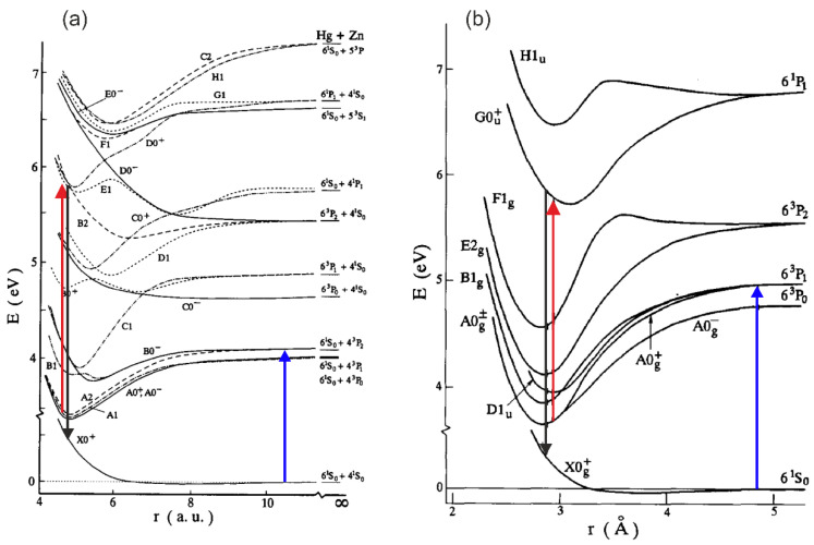
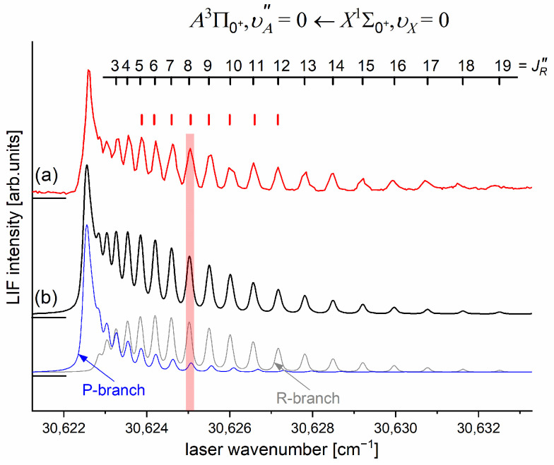
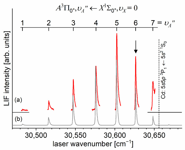
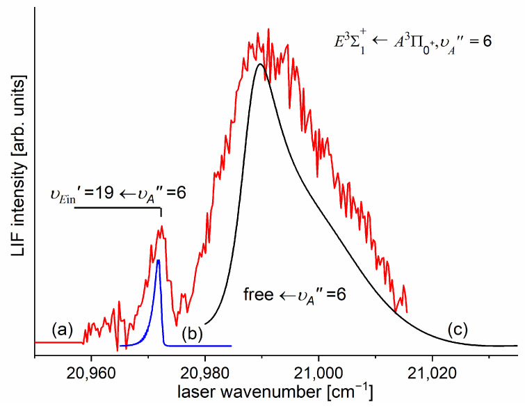
Recent progress in studies of Rydberg double-well electronic energy states of MeNg (Me = 12-group atom, Ng = noble gas atom) van der Waals (vdW) molecules is presented and analysed. The presentation covers approaches in experimental studies as well as ab initio-calculations of potential energy curves (PECs). The analysis is shown in a broader context of Rydberg states of hetero- and homo-diatomic molecules with PECs possessing complex 'exotic' structure. Laser induced fluorescence (LIF) excitation spectra and dispersed emission spectra employed in the spectroscopical characterization of Rydberg states are presented on the background of the diverse spectroscopic methods for their investigations such as laser vaporization-optical resonance (LV-OR), pump-and-probe methods, and polarization labelling spectroscopy. Important and current state-of-the-art applications of Rydberg states with irregular potentials in photoassociation (PA), vibrational and rotational cooling, molecular clocks, frequency standards, and molecular wave-packet interferometry are highlighted.

Keywords: Rydberg electronic state; ab initio calculations; double-well potential; rotational energy structure; van der Waals molecule; vibrational energy structure.


Conflict of interest statement

The authors declare no conflicts of interest.

Figures

Figure 26
Figure 26
Experimental LIF excitation spectra terminating at the vibrational energy structure of the E3Σ1+-state inner potential well in CdKr, recorded using (a) E3Σ1 in+,υEinA3Π0+,υA=9 and (c) E3Σ1 in+,υEinB31,υB=1 transitions, with intensities of the spectrum in (a) normalized because of the large spectral region in which the total spectrum for υEin was recorded (different dye lasers and carrier gas pressures were applied). (b) Simulation of positions only and (d) simulation of positions and intensities performed assuming the E3Σ1 in+ potential representation as the result of the IPA method using the (b) LEVEL [205] and (d) LEVEL and PGOPHER [206] programs, assuming (d) Trot=3 K and ΔL=ΔG=0.15 cm1. (e) B-S plot for the υEin=021υA=6 (full squares) and υEin=2228υB=1 (empty squares) progressions, showing distinct nonlinearity for υEin24. The size of the points in the plot equals the error bars for ΔG.
Figure 1
Figure 1
Illustration of the anti-crossing (avoided crossing) of the U1 and U2 potential energy curves that causes the formation of a potential energy barrier in the U2 separating two, inner and outer, potential wells.
Figure 2
Figure 2
(a) Cd+ e interaction potential and square of the module of Ψ6s atomic orbital of Cd based on the results of ab initio calculations taken from Ref. [4], where values of the orbital are in arbitrary units (they do not correspond to the values on vertical axis); (b) energy shift Es(R) due to the Rydberg electron e–Ng interaction calculated using Equation (1) for the E3Σ1+ Rydberg state of CdNg molecules; (c) charge Me+–induced-dipole (Ng) interaction energy representing the dominating contribution to the long-range Me+–Ng interaction; and (d) ab initio-calculated PECs of the E3Σ1+ state of CdNg taken from Refs. [39,40]. The dashed vertical line in (a) and (b) indicates the classical range of the Rydberg 6s electron. Note: 1 a.u.(1 bohr) = 0.5292 . For details, see text.
Figure 3
Figure 3
Photoassociation from the rubidium 5s 2S1/2 ground state asymptote [reaction (1) and (1’)] to (a) a typical long-range attractive potential; (b) a double-well potential, attractive at a long distance [e.g., 0g(5p 2P3/2)]; and (c) a double-well potential, repulsive at a long distance [e.g., 0g+(5p 2P3/2)]. The system decays by spontaneous emission either back to the continuum [reaction (2)] or to a bound level of a lower electronic state [reaction (3)] [e.g., the a3Σu+(5s 2S1/2) state]. For case (a), reaction (3) is usually unlikely. Note: 1 a.u.(1 bohr) = 0.5292 . (from Ref. [89], under permission of EDP Sciences, Springer-Verlag).
Figure 4
Figure 4
Illustration of optical–optical double resonance (OODR) method applied in molecular excitation. Potential energy curves (PECs) (solid lines) of the X1Σ0+(5s2 1S0), A3Π0+5s5p 3P1, B315s5p 3P1, and E3Σ1+5s6s 3S1 states in CdAr and electronic transition dipole moments squared TDM2(R) (dashed lines) are plotted according to the recent result published by Krośnicki et al. [4]. TDM2 are plotted for (a) the first step of OODR: the A3Π0+X1Σ0+ and B31X1Σ0+ transitions, and (b) the second step of OODR: the E3Σ1+A3Π0+ and E3Σ1+B31 transitions. Examples of vibrational transitions (a) υA,BυX=0 and (b) υEυA,B used in OODR are shown with vertical lines. The intensity of the vibrational transition depends on TDM2ψelμelψeldτel2 along with so-called overlap integrals (a) ψυψυdR and (b) ψυψυdR for the first and second transition, respectively, where μel is an electric dipole operator, ψel are electronic eigenfunctions, and ψυ are υ-level vibrational eigenfunctions (shown for each vibrational level). (c) Details of the second excitation. The ab initio-calculated height of the potential barrier is somewhat larger than that obtained from an experiment. Experimental positions of the υEin and υEout and υA,B levels are also depicted.
Figure 5
Figure 5
Diagram of interatomic potentials for (a) HgZn (from Ref. [153], under permission of Elsevier Science B.V.) and (b) Hg2 (from Ref. [72], under permission of Elsevier Science B.V.) showing the relevant pump (blue arrows), probe (red arrows), and LIF (black arrows) processes. Arrows are added to the original figure. Note: 1 a.u. = 0.5292 .
Figure 6
Figure 6
The ‘V-scheme’ of polarization labelling spectroscopy (see the text for details).
Figure 7
Figure 7
LIF excitation spectrum recorded using the A3Π0+,υAX1Σ1+,υX=0 and B31,υBX1Σ1+,υX=0 transitions in CdNe, as reported in Ref. [203], the former being first step of the excitation in the OODR process E3Σ1+,υA3Π0+,υAX1Σ1+,υX=0, which allowed for investigating the E3Σ1+-state potential and, partly, potential barrier. The arrow shows the υA=0,1 that was used as the origin for the second transition in OODR. The asterisk depicts the vibrational band recorded in higher resolution and shown in Figure 8.
Figure 8
Figure 8
(a) LIF excitation spectrum showing the profile of the vibrational component recorded using the A3Π0+,υA=0,JRX1Σ0+,υX=0,J first OODR transition in CdNe. (b) Simulation performed using LEVEL [205] and PGOPHER [206] programs allowed for determining the JR assignment shown above the spectrum, which reveals the partly resolved structure of the R-branch (P-branch is also shown). In the simulation, Trot=5 K (rotational temperature) and ΔL=ΔG=0.1 cm1 were assumed (Lorentzian and Gaussian broadenings responsible for laser bandwidth and transversal divergence of molecular beam, respectively) as well as Morse representations of the A3Π0+- and X1Σ0+-state potentials from Ref. [203]. The positions of the JR levels used as the intermediates in the OODR process (red ticks, compare with Figure 9) and a ±10 cm1 vertical bar representing the laser bandwidth are depicted.
Figure 9
Figure 9
Branches of rotational transitions involved in the realization of the selective J excitation in the OODR experiment performed in CdNe using the E3Σ1+,υE=0,JA3Π0+,υA=0,JRX1Σ0+,υX=0,J transition paths. Details are provided in the text.
Figure 10
Figure 10
(a) LIF excitation spectra recorded using the E3Σ1+,υE=0,JA3Π0+,υA=0,JR second OODR transition in CdNe, for JR=5,,12 selected in the A3Π0+,υA=0,JRX1Σ0+,υX=0,J first OODR transition (see also Figure 9). (b) Separations Δ(JR) between energies of rotational transition recorded for the P(JR1) and R(JR+1) branches. Linear regression allowed for determining the Bυ=0 rotational constant.
Figure 11
Figure 11
(a) Partly rotationally resolved profiles of vibrational bands recorded in the LIF excitation spectra of the E3Σ1+,υEA3Π0+,υA second-step OODR transitions in CdNe. (b) Simulations performed using the LEVEL [205] and PGOPHER [206] programs: P-, Q-, and R-branches are shown. The intensity of Q-branch is damped, as concluded in Ref. [10]. All simulations are performed assuming Trot=5 K, ΔL=ΔG=0.15 cm1, Jmax=69 depending on the transition and the isotopic shift between CdNe isotopologues (abundances > 3%) included in the simulation as approximately one order of magnitude smaller than their rotational structure.
Figure 12
Figure 12
The E3Σ1+(5s6s 3S1) Rydberg state potential well of CdNe determined experimentally [10,11] (black solid line) represented with a Morse function compared with the results of ab initio calculations from Czuchaj and Stoll [6] (blue: empty triangles and line), Czuchaj et al. [7] (green: empty squares and line), and Krośnicki and collaborators [39,40] (red: empty circles and line). Positions of υ levels supported by the potential well are depicted: Eυ=0=51,542 cm1, Eυ=1=51,581 cm1, Eυ=2=51,602.5 cm1 as observed in the experiment. The energy limit beyond which no boundbound transitions were observed is depicted.
Figure 13
Figure 13
(a) LIF excitation spectrum recorded using the A3Π0+,υAX1Σ1+,υ=0 transition in CdAr, being first step of excitation in the OODR process E3Σ1 in+,υEinA3Π0+,υAX1Σ1+,υ=0, which allowed for investigating the E3Σ1in+-state inner well and, partly, potential barrier. (b) Simulation performed using the LEVEL [205] and PGOPHER [206] programs and data derived from the analysis of the experimental spectrum [13]. The arrow shows the υA=6 that was used as the origin for the second transition in OODR. Also, the υA=6υ=0 band recorded with higher resolution was used, among others, in the isotopologue selection experiment (see Section 5.4). The position of the atomic transition in Cd is depicted.
Figure 14
Figure 14
(a) LIF excitation spectrum of the υEin=019υA=6 progression recorded using E3Σ1 in+A3Π0+ in CdAr. (b) Simulations performed using a representation of the E3Σ1+-state inner well (b) obtained from the IPA method and (c) using a Morse function. As the figure compares only the positions of the vibrational components, their intensities in (ac) were normalized. To make the comparison easier, several last υEinυA=6 components are shown on different horizontal scales. Details of the υEin=19υA=6 component, shown in the rectangular frame. (d) B-S plot for the υEin=019υA=6 progression presenting a distinct nonlinearity for approx. υEin>12.
Figure 15
Figure 15
Comparison of the E3Σ1+5s6s 3S1-state inner well IPA representation in CdAr (black: full circles and line) with the results of the most recent ab initio calculations by Krośnicki et al. [4] (red: full circles and line) and ab initio calculations by Czuchaj and Stoll [6] (blue: empty triangles and line), Czuchaj et al. [7] (green: empty squares and line), and Krośnicki and collaborators [39,40] (red: empty circles and line). The inset shows vicinity of the potential barrier that separates the inner and the outer wells. The position of three υEin levels closest to the dissociation energy is shown. The height of the potential barrier Eb is as estimated in Ref. [13] (grey rectangle) and as determined in Ref. [12] (horizontal black line) (also see Table 1).
Figure 16
Figure 16
(a) LIF excitation spectrum recorded using the E3Σ1+A3Π0+ transition in CdAr [13], showing the last υEin=19υA=6 quasi-boundbound transition and profile of freebound transitions starting from υA=6. (b) and (c) Simulations of the boundbound and freebound transitions performed using the PGOPHER [206] and BCONT [209] programs, respectively.
Figure 17
Figure 17
(A) Partly rotationally resolved profiles of vibrational bands recorded in the LIF excitation spectrum of the E3Σ1 in+,υEinA3Π0+,υA=6 second-step OODR transition in 116Cd40Ar (with a small admixture of 114Cd40Ar). (a) Experimental spectra. (b) Simulations performed using the LEVEL [205] and PGOPHER [206] programs assuming Trot=2.5 KυEin=2 and 5,Trot=3.5 KυEin=11, Trot=5 K (υEin=17), and ΔL=ΔG=0.1 cm1. (c) Intensities of rotational P-, Q- and R-branches contributing to (b), depicted with a colour code in part for υEin=17. The intensity of the Q-branch is damped, as concluded in Ref. [10]. (B) The profile of the A3Π0+,υA=6X1Σ1+,υ=0 first-step OODR transition showing the possibility of selective excitation of 116Cd40Ar with a small admixture of 114Cd40Ar isotopologue (see also Section 5.4). (a) Experimental LIF excitation spectrum, (b) total simulation of the profile, and (c) contributions to the total simulated profile corresponding to different CdAr isotopologues. Vertical blue dashed line and wide bar depict a laser wavenumber of the first-step OODR transition and the laser bandwidth, respectively.
Figure 18
Figure 18
The E3Σ1 out+,υEoutB31,υB=2 vibrational band of CdAr. (a) Experimental spectrum. Simulations performed using the PGOPHER program [206] assuming that (b) Re out = 7.63 [16] and (c) Re out = 6.90 were obtained as a result of the new method of bond length adjustment with the help of the CRe out agreement parameter [15]. In both simulations, Trot=5 K and ΔL=ΔG=0.1 cm1 were used. Note: according to later studies, the figure shows the wrong υEout assignment as it lacks the low-intensity υEout=0υB=2 component that was recorded during the investigation of the E3Σ1 out+,υEoutB31,υB transitions [12], causing correction of the spectroscopical characterization of the E3Σ1 out+ well. This is also illustrated in Figure 19 and Figure 20.
Figure 19
Figure 19
The CRe out agreement coefficient describing the agreement between Iexpt(i) experimental and Isimi(Re out) simulated intensities of the vibrational components in the LIF excitation spectrum recorded using the E3Σ1out+,υEoutB31,υB transition (see Equation (2)) for υB=1 (black full circles and line) [15] and υB=2 (black empty circles and line) [15]. The plot is supplemented with the recent results of Ref. [12], which concluded in the correction of the υEout assignment (see Section 5.2.3) for υB=1 (grey squares and line), υB=2 (green squares and line), υB=3 (blue squares and line), and υB=4 (red squares and line). Symbols with error bars and corresponding rectangles depict the Re out results of Refs. [12,15] and, for comparison, Ref. [16].
Figure 20
Figure 20
The (ωeωexe) agreement plot drawn according to Equation (3), expressing simulation-to-experiment agreement with respect to the E3Σ1out+ state of CdAr using LIF excitation spectra of the E3Σ1out+,υEoutB31,υB transitions for (a) υB=1, as in Ref. [15], and (b) υB=3, as in Ref. [12], after recording an additional component in the spectrum and correction of the υEout assignment (see Section 5.2.3). The plot shows the dependency between ωe and ωexe vibrational constants. Error bars: uncertainties in ωe and ωexe, as in Ref. [16] (red), Ref. [15] (yellow), and, finally, Ref. [12] (white).
Figure 21
Figure 21
LIF excitation spectrum recorded using the B31,υBX1Σ1+,υX=0 transition in CdAr, as reported in Ref. [210], which is the first step of excitation in the OODR process that allowed for investigating the E3Σ1 out+-state outer well [12,15] and potential barrier [12] using the E3Σ1 out+,υEoutB31,υB second-step OODR transition. Arrows show υB values that were used as origins in the second-step transition.
Figure 22
Figure 22
LIF excitation spectra (red lines) recorded using (a) the E3Σ1 out+,υEoutB31,υB=04 boundbound and (b) the E3Σ1+B31,υB=04 freebound transitions in CdAr, and their respective simulations [205,206,209] (black lines). The position υEout=0υB component that was not previously recorded [15] is depicted (one asterisk). The position of the E3Σ1 in+,υEin=1719B31,υB vibrational components is shown, proving that the spectrum also contains transitions to the E3Σ1+-state inner well. Unlike in other spectra recorded using second-step OODR transition and presented in this review, here, laser wavenumbers are given with respect to the X1Σ1+-state asymptote. The energy corresponding to the 5s6s 3S1 Cd asymptote is depicted (vertical dashed line). The inset to (a) shows details of the very weak υEoutυB=0 boundbound transitions with clearly visible υEin=18υB=0. (c) B-S plot for υEoutυB=4 progression and with corrected υEout assignment, providing final values for the E3Σ1 out+ outer well vibrational constants ωe=4.36 cm1 and ωexe=0.207 cm1.
Figure 23
Figure 23
Comparison of the CdAr interatomic potential of the E3Σ1+(5s6s 3S1) Rydberg-state outer well representations close to the dissociation limit, being the result of series of experiments using the OODR excitation method as follows: very first investigation by Koperski and Czajkowski [17] (grey dashed-dotted line), result of Urbańczyk and Koperski [15] (grey dotted line), and the most recent result of Sobczuk et al. [12] (black solid line)—also see Table 1. Note: for the inner potential well, the representations refer to Figure 15. Part of the whole E3Σ1+-state potential representation in the vicinity of the potential barrier as the result of Ref. [12] is also shown (blue line and points)—see the text for details. The ab initio-calculated potential by Krośnicki et al. [4] is shown for comparison (red line and points). The potential of the B31 intermediate state [16] used in the OODR process is also drawn (green solid line). Three ways to execute the excitation using the E3Σ1+B31,υB=4 transitions are depicted with vertical arrows as follows: (a) quasi-boundbound to the E3Σ1 in+, (b,c) freebound terminating at the inner and outer repulsive walls of the potential barrier, respectively, and (d) boundbound to the E3Σ1 out+.
Figure 24
Figure 24
(a) Ab initio-calculated interatomic potentials of CdAr electronic energy states [4] used to illustrate the OODR process of the excitation of E3Σ1+,υEin=2 from X1Σ1+,υX=0 via A3Π0+,υA=5 (vertical solid arrows) followed by emission to several lower-lying molecular states, allowing for the characterization of their potentials using bound→free and bound→bound transitions. (b) Examples of simulated dispersed emission spectra [205,206,209] with bound→free (b→f) and bound→bound (b→b) transitions from E3Σ1+,υEin=2 to c3Σ1+(5s5p 3P2), b3Π2(5s5p 3P2) and a3Π0(5s5p 3P0) electronic ‘dark’ states, which would serve as data to determine their PECs [202].
Figure 25
Figure 25
LIF excitation spectra recorded using the (a) A3Π0+,υAX1Σ1+,υX=0 [215] and (b) B31,υBX1Σ1+,υX=0 [106] transitions in CdKr, both being the first steps of the excitation in OODR processes, i.e., E3Σ1 in+,υEinA3Π0+,υAX1Σ1+,υX=0 and E3Σ1+,υEB31,υBX1Σ1+,υX=0, that allowed for investigating the inner E3Σ1 in+ and outer E3Σ1 out+ potential wells. Arrows show the υA=9 and υB=0, 1, 4, 6 that were used as origins for the second-step OODR transition. The asterisk depicts the υA=9υX=0 vibrational band recorded with higher resolution and used, among others, in the isotopologue selection experiment (see Section 5.4). Note: irregular, i.e., non-Morse, behaviour of υB levels is due to the double-well character of the B31-state potential [106].
Figure 27
Figure 27
LIF excitation spectra (red traces) terminating at the υEout vibrational energy structure of the E3Σ1+-state outer well and the most upper-lying υEin levels of the E3Σ1+-state inner well in CdKr, recorded using E3Σ1 out+,υEoutB31,υB and E3Σ1 in+,υEinB31,υB, respectively, starting at (a) υB=0, (b) υB=1, (c) υB=4, and (d) υB=6. Simulations of the E3Σ1 out+B31 and E3Σ1 in+B31 spectra (blue and grey traces, respectively) performed using the LEVEL [205] and PGOPHER [206] programs in which E3Σ1 out+, E3Σ1 in+ and B31-state representations were taken from Refs. [19,106], and Trot=3 K and ΔL=ΔG=0.15 cm1 were assumed. (e) B-S plot drawn for the E3Σ1 out+ potential well in CdKr based on the E3Σ1 out+,υEoutB31,υB=6 transition shown in (d), in which strong nonlinearity is present, and two regions, A (υEout=08) and B (υEout=916), each of linear behaviour, can be extracted.
Figure 28
Figure 28
Representations of the E3Σ1+(5s6s 3S1) Rydberg state potential of CdKr with an inset showing details of the potential barrier and outer potential well close to the dissociation limit. E3Σ1 in+ (red line and circles) and E3Σ1 out+ (red line and squares) potential well representations as results of the IPA methodology and analysis of the spectra in Figure 26a,c and Figure 27d, respectively. A Morse representation of E3Σ1 in+, being the result of the B-S plot analysis in Figure 26e, is also presented (blue solid line). The experimentally determined representations are compared with two results of ab initio calculations [216], showing their considerable difference, including those from 2008 performed by Krośnicki and collaborators [39,40] (black line and empty circles) and those most recently performed by Krośnicki et al. [208] (black line and full circles). The estimated height of the potential barrier Eb is shown as a red horizontal line. For comparison, the result of the first experimental study [20] (grey solid lines) is included. The ranges of υEin and υEout excited from B31,υB and analysed in [19] are shown (grey rectangles).
Figure 29
Figure 29
(A): (a) Profile of the LIF excitation spectrum recorded using the A3Π0+,υA=9X1Σ1+,υ=0 transition in CdKr. (b) Total simulation of the profile performed using the PGOPHER [206] program, assuming Trot=4 K and ΔL=ΔG=0.1 cm1 as well as Bυ and Dυ rotational constants, and transition energies calculated using the LEVEL [205] program for the A3Π0+ [16] and X1Σ1+-state [215] potential characteristics. (c) Individual contributions to (b) that originate from different CdAKrACdKr isotopologues with abundances larger than 1%. (d) Positions of the νlas 1 laser wavenumber of OODR first-step excitation used in (B); examples of νlas 1±0.1 cm1 are represented with blue vertical dashed lines and rectangles. (B): Profiles of LIF excitation spectra recorded using the E3Σ1in+,υEin=18A3Π0+,υA=9 OODR second-step transition for different νlas 1±0.1 cm1 depicted in (A)-(d), i.e., for different combinations of excited CdAKrACdKr isotopologues. For the simulation shown with the black line (in position-2), refer to (C). (C): (a) Profiles of LIF excitation spectra recorded using the E3Σ1in+,υEin=0,3,18A3Π0+,υA=9 transitions in 114Cd86Kr (with small admixture of 116Cd40Kr)—excitation in position-2: νlas 1=30,557.58±0.1 cm1 shown in (A). (b) Simulations performed using the PGOPHER [206] program, assuming JA min=0, JA max=15, Trot=4 K (for υEin=0 and 3), Trot=15 K (forυEin=18), and ΔL=ΔG=0.1 cm1, as well as Bυ and Dυ rotational constants, and transition energies calculated using the LEVEL [205] program for the E3Σ1in+ [16] and A3Π0+-state [16] potential characteristics. (c) Simulated distributions of P-, Q-, and R-branch components depicted with a colour code as in part for υEin=0. The intensity of the Q-branch is damped, as concluded in Ref. [10].
Figure 30
Figure 30
(a) Scheme of the double-resonance technique for the detection of the ‘dark’ intermediate υ vibrational levels of the c31 state in HgAr using probe laser excitation to the potential barrier in the E31 Rydberg state. (b) c31υ X10+(υ=0) excitation spectrum of the HgAr vdW complex plotted against the pump wavenumber (from Ref. [25], under the permission of the American Institute of Physics).
Figure 31
Figure 31
Pump control probe scheme for detecting the populations of the A30+, υA vibrational levels created by a double-laser pulse from the X10+, υX=0 vibrational level (from Ref. [217], under the permission of the American Physical Society).
Figure 32
Figure 32
Dispersed emission spectrum corresponding to the B315s5p 3P1,υ=4 X1Σ0+5s2 1S0,υ transitions in the CdAr molecule (a) recorded using a SpectraPro HRS 750 spectrometer (Teledyne Princeton Instruments) equipped with a CCD camera with an image intensifier (PIMAX 4) and diffraction grating with 1200 grooves/mm. (b) Simulation of the dispersed emission spectrum from (a) performed using the LEVEL [205] and PGOPHER [206] programs and assuming parameters of the B31 and X1Σ0+-state potentials from Refs. [14,218], respectively, as well as Gaussian broadening responsible for spectrometer spectral throughput ΔG=38 cm1. (c) Simulation of the recorded background signal associated with the excitation laser beam at the B31,υ=4X1Σ0+,υ=0 transition. (d) Simulated [205,206] distribution of transitions to different υ values in the X1Σ0+ ground state originating from υ=4 in the B31 state performed for ΔG=1.9 cm1.

Similar articles

References

    1. von Neumann J., Wigner E.P. Über das Verhalten von Eigenwerten bei adiabatischen Prozessen. Phys. Z. 1929;30:467–479. doi: 10.1007/978-3-662-02781-3_20. - DOI
    1. Dressler K. In: Photophysics and Photochemistry above 6 eV. Lahmani F., editor. Elsevier; Amsterdam, The Netherlands: 1985. pp. 327–341.
    1. Kędziorski A., Zobel J.P., Krośnicki M., Koperski J. Rydberg states of ZnAr complex. Mol. Phys. 2022;120:e2073282. doi: 10.1080/00268976.2022.2073282. - DOI
    1. Krośnicki M., Kędziorski A., Urbańczyk T., Koperski J. Rydberg states of the CdAr van der Waals complex. Phys. Rev. A. 2019;99:052510. doi: 10.1103/PhysRevA.99.052510. - DOI
    1. Czuchaj E., Krośnicki M., Stoll H. Quasirelativistic valence ab initio calculation of the potential curves for the Zn-rare gas van der Waals molecules. Chem. Phys. 2001;265:291–299. doi: 10.1016/S0301-0104(01)00323-8. - DOI

LinkOut - more resources