Neural Correlates of Category Learning in Monkey Inferior Temporal Cortex

Abstract

Area TE is required for normal learning of visual categories based on perceptual similarity. To evaluate whether category learning changes neural activity in area TE, we trained two monkeys (both male) implanted with multielectrode arrays to categorize natural images of cats and dogs. Neural activity during a passive viewing task was compared pre- and post-training. After the category training, the accuracy of abstract category decoding improved. Single units became more category selective, the proportion of single units with category selectivity increased, and units sustained their category-specific responses for longer. Visual category learning thus appears to enhance category separability in area TE by driving changes in the stimulus selectivity of individual neurons and by recruiting more units to the active network.

Keywords: area TE; categorization; electrophysiology; inferotemporal cortex; monkey; vision.

Figure 1.

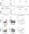
A, Diagram of the passive viewing task. In brief, monkeys were required to fixate on the central fixation square while five images were presented in succession, followed by a liquid reward and an intertrial interval. See Materials and Methods for details. B, Diagram of the category training and transfer test task. In brief, in each trial, monkeys were required to release a touch bar in one of two intervals to indicate whether the image on screen was a cat or a dog. To correctly respond to a cat stimulus, monkeys had to release during the interval in which the central fixation square was red, which allowed them to avoid a timeout; to correctly respond to a dog stimulus, monkeys had to hold the bar through the red period and release when the square turned green, which resulted in a liquid reward. See Materials and Methods for details. C, Schematic of the experimental timeline. Neural activity was compared before and after monkeys learned to categorize natural images of cats and dogs. Monkeys were trained with 40 images and tested using 480 similar held-out images. All passive viewing sessions used all 520 images, randomly interleaved in blocks. D, The 40 images used for training. E, A random subset of 40 of the 480 images used for the transfer test. F, Behavioral data from the category training, colored by session number; i, fraction correct trials per session sextile; ii, same as i but for the first 480 completed trials of the transfer testing session, in which monkeys had only one opportunity to categorize each test image; iii, session averages for the data shown in i and ii; iv, median (±IQR) reaction times for correct cat trials (release-on-red cat trials, see Materials and Methods), which correspond approximately to the time it takes monkeys to categorize the image (Eldridge et al., 2018). Note the increased reaction times on the transfer test day, indicating nonexpertise.

Figure 2.

A, Distributions of the HSV values of pixels in the 520 cat/dog images. Only foreground pixels were considered. The foreground was extracted using a k-means clustering algorithm (k = 6) and removing the white component. B, Analysis of object size (number of foreground pixels) and image-mean relative luminance. C, Frequency components of the cat and dog stimuli.

Figure 3.

A, i, Utah array locations in both monkeys, ii number of single units recorded from each pre-/post-training session, from each Utah array. B, Distribution of Fano factors for all single units on pre- and post-training days. Carat and line denote mean ± standard deviation. C, Distribution of the maximum-image-average evoked firing rates for all single units pre- and post-training. Carat and line denote median ± IQR. D, Smoothed firing rates for four example category-selective neurons from each monkey. Subsequent analyses were performed on raw spike counts in selected windows, except where noted (Fig. 7).

Figure 4.

A, Time course of the accuracy of abstract category SVM decoders (see Materials and Methods), trained on neural population response vectors (spike counts in each 100 ms bin; mean ± shaded SEM). Bouts of significant pre- versus post-training difference were determined with t tests and a cluster-based permutation procedure that uses trial-shuffled spike counts (Wittig et al., 2018; *p < 0.05). B, Same as A but with data from each individual array. C, Accuracy of the abstract category SVM decoders in the 175–275 ms bin, across full-image-set baseline and experimental sessions (mean ± SEM). D, same as C, but for the initial 20/20 baseline sessions. E, Accuracy of abstract category SVM decoders in the 175–275 ms bin, with increasing numbers of the top 100 units used for training (see Materials and Methods). Vertical lines denote half-maximal accuracy for pre- (blue) and post-training (red), respectively. See Table 1 for parameters of the sigmoidal fits.

Figure 5.

A, Fraction of single units significant in a GLM regressing image category versus spike count 175–275 ms after image onset, before and after category training. B, Same as A, with data from each individual array. C, Same as A but across experimental sessions. D, Distribution of significant coefficients from the regressions. Carat and line represent mean ± standard deviation. ^#p < 0.1.

Figure 6.

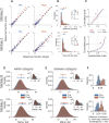
A, All single units’ responsiveness to cats or dogs, across sessions, as measured by the fraction of images from each category that evoked a significant visual response. Black dotted line, unity; red line, best-fit line from major-axis regression. B, Distributions of the category selectivity shown in A, summarized for each unit by the absolute difference between the fraction of cat and dog images evoking a significant response. Carat and line above the histograms represent mean and SD, respectively (*p < 0.05; **p < 0.01; ***p < 0.001). B, Inset, estimated slope (from major-axis regression; mean + 95% confidence intervals) for best-fit lines in B. C, Cumulative distribution of sparseness of single unit responses to either cats or dogs, as measured by the sparseness index from Vogels (1999). D, Pairwise Mahalanobis distances for all within-category trial pairs. Inset shows the same data on a log scale to highlight (lack of) outliers. E, Same as D but for between-category trial pairs. F, Pre- and post-training bootstrap distributions for the difference between the medians of the between-category versus within-category pairwise Mahalanobis distance distributions.

Figure 7.

A, Accuracy of abstract category SVM decoders, trained and tested on neural population response vectors from different timepoints. The same set of top 100 units was used for all train/test combinations. B, Time courses of significant difference of category-averaged responses for all units. Each row represents a single unit. Yellow represents significance (see Materials and Methods; p < 0.01). C, Probability distribution for the durations of all single unit time courses (not including zero duration) of significant single-unit category coding from the analysis in B (*p < 0.05; ***p < 0.001, one-sided rank-sum test). D, Net proportion of units showing a significant difference at each timepoint in B. Marks above the data represent significant pre versus post difference (two-sided chi-square test, p < 0.05). Dotted lines indicate first instance of a proportion significantly different from zero (two-sided chi-square test, p < 0.05).

References

1. Afraz S-R, Kiani R, Esteky H (2006) Microstimulation of inferotemporal cortex influences face categorization. Nature 442:692–695. 10.1038/nature04982 - DOI - PubMed
1. Anon (n.d.) Web content accessibility guidelines (WCAG) 2.0. Available at: https://www.w3.org/TR/WCAG20/. Accessed October 30, 2023.
1. Baene WD, Ons B, Wagemans J, Vogels R (2008) Effects of category learning on the stimulus selectivity of macaque inferior temporal neurons. Learn Mem 15:717–727. 10.1101/lm.1040508 - DOI - PubMed
1. Bao P, She L, McGill M, Tsao DY (2020) A map of object space in primate inferotemporal cortex. Nature 583:103–108. 10.1038/s41586-020-2350-5 - DOI - PMC - PubMed
1. Bowman EM, Aigner TG, Richmond BJ (1996) Neural signals in the monkey ventral striatum related to motivation for juice and cocaine rewards. J Neurophysiol 75:1061–1073. 10.1152/jn.1996.75.3.1061 - DOI - PubMed
LinkOut - more resources