Performance of a Radio-Frequency Two-Photon Atomic Magnetometer in Different Magnetic Induction Measurement Geometries

Abstract

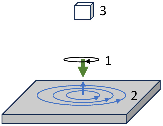
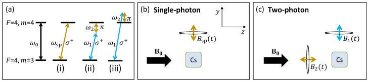
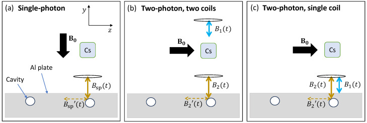
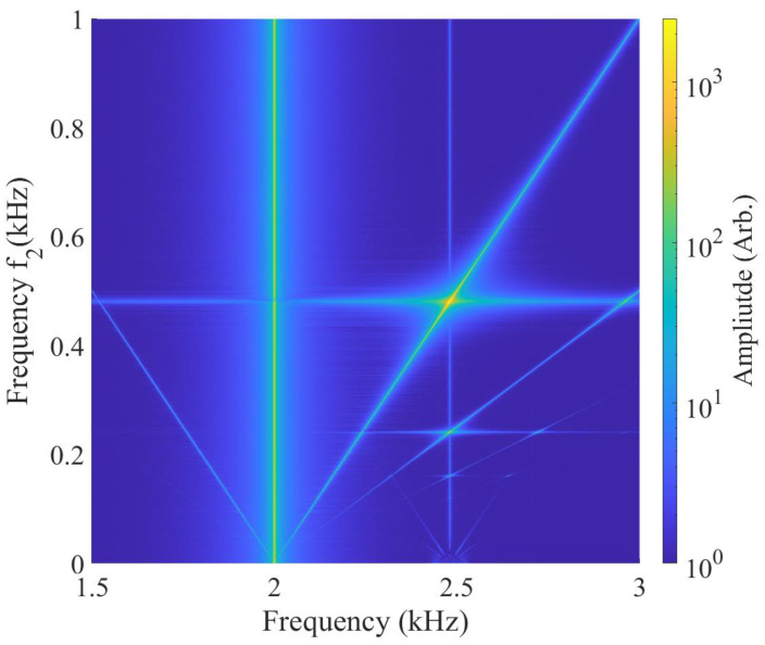
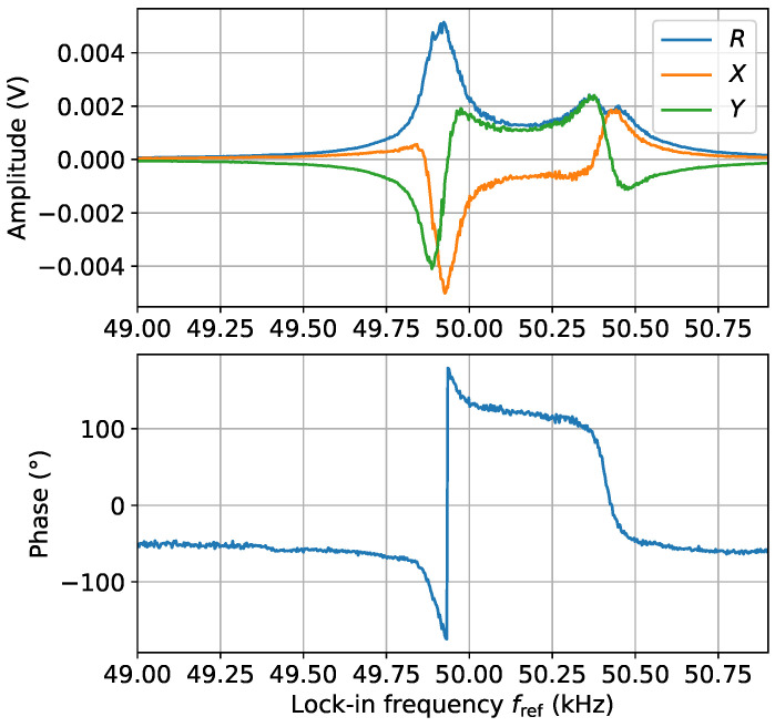
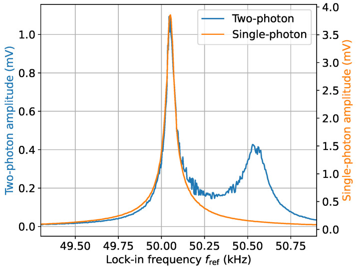
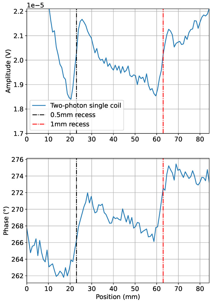
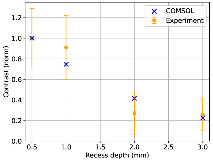
Measurements monitoring the inductive coupling between oscillating radio-frequency magnetic fields and objects of interest create versatile platforms for non-destructive testing. The benefits of ultra-low-frequency measurements, i.e., below 3 kHz, are sometimes outweighed by the fundamental and technical difficulties related to operating pick-up coils or other field sensors in this frequency range. Inductive measurements with the detection based on a two-photon interaction in rf atomic magnetometers address some of these issues as the sensor gains an uplift in its operational frequency. The developments reported here integrate the fundamental and applied aspects of the two-photon process in magnetic induction measurements. In this paper, all the spectral components of the two-photon process are identified, which result from the non-linear interactions between the rf fields and atoms. For the first time, a method for the retrieval of the two-photon phase information, which is critical for inductive measurements, is also demonstrated. Furthermore, a self-compensation configuration is introduced, whereby high-contrast measurements of defects can be obtained due to its insensitivity to the primary field, including using simplified instrumentation for this configuration by producing two rf fields with a single rf coil.

Keywords: atomic magnetometer; magnetic induction tomography; non-destructive testing.

Figure 1

Model of the generic configuration of an inductive measurement. An excitation field (1), the so-called primary rf field and represented by the green arrow, drives the object response (2), which in this case is the generation of eddy currents denoted by the blue circles. These produce a secondary rf field, represented by a blue arrow. The resultant field is detected by a sensor (3), depicted by the white box.

Figure 2

(a) Detection of the rf field with an atomic magnetometer is performed by monitoring the amplitude and phase of the atomic coherence driven by the rf field between Zeeman sublevels of the $F=4$ caesium ground state. For simplicity, only two sublevels are shown. In the single-photon case in [a(i)], the transition frequency ${\omega }_0$ is tuned into resonance with the detected rf field frequency ${\omega }_{\mathrm{sp}}$ by adjusting the bias magnetic field ${\mathbf{B}}_0$. The sensor detects only the circularly polarised component (${\sigma }^{+}$) of the rf field. In the two-photon case, the atomic coherence is driven by two rf fields. The resonance condition is met by the [a(ii)] sum or [a(iii)] difference in the field frequencies. Selection rules set the conditions for the polarisations of the fields. The gold coloured arrows represent the field that drives the response of interest (low frequency) from the object relevant to the inductive measurements. The choice of frequency and field polarisation used is described in Section 3.4. (b) The single-photon resonance condition can be satisfied when an rf field ${\mathbf{B}}_1\left(t\right)$ is applied perpendicularly to ${\mathbf{B}}_0$ with ${\omega }_{\mathrm{sp}}={\omega }_0$. (c) In the two-photon configuration, an extra rf field ${\mathbf{B}}_2\left(t\right)$ is required along the bias field axis such that a two-photon transition can be achieved.

Figure 3

MIT experimental setups for the (a) single-photon, (b) two-photon two-coil, and (c) two-photon single-coil configurations. The gold coloured arrows represent the field that drives the response of interest (low frequency) from the object relevant to the inductive measurements. (a) In the single-photon self-compensation case, the bias field is directed along the primary field ${\mathbf{B}}_{\mathrm{sp}}\left(t\right)$ (double-ended gold arrow), and the magnetometer is sensitive to secondary fields ${\mathbf{B}}_{\mathrm{sp}}^{\prime }\left(t\right)$ in the 2D plane perpendicular to ${\mathbf{B}}_0$. (b) In the two-photon two-coil configuration, the high-frequency auxiliary coil producing ${\mathbf{B}}_1\left(t\right)$ is far from the plate. The low-frequency rf field ${\mathbf{B}}_2\left(t\right)$ can penetrate through the material due to its large skin depth, and the secondary field ${\mathbf{B}}_2^{\prime }\left(t\right)$ induced parallel to the surface of the plate is measured by the sensor. The optimal geometric configuration is chosen due to the $1/{\omega }_2$ amplitude dependence of the two-photon coherence, described in Section 3.3. (c) In the two-photon single-coil case, both frequency components come from the same coil. Only the low-frequency component will produce a secondary field ${\mathbf{B}}_2^{\prime }\left(t\right)$ along the bias field due to the attenuation of the high-frequency rf field at the object’s surface.

Figure 4

FFTs of the polarisation rotation signal recorded as $f_2$ are scanned over the 0–1 kHz frequency range, whilst $f_1$ remains fixed at 2 kHz in shielded conditions. The two-photon profiles are represented by the diagonal lines, $f_1\pm f_2$. Atomic shot noise produces a weak signal at the resonant frequency $f_0=2.48$ kHz. The two-photon resonance can be observed when $f_0=f_1+f_2$.

Figure 5

The in-phase (X), quadrature (Y), and magnitude (R) components of the lock-in are monitored during the two-photon resonance signal, demonstrating that phase information $\varphi =arctan(Y/X)$ can be obtained in a two-photon measurement. The two-photon transition can be observed at $f_{\mathrm{ref}}=f_0=49.9$ kHz ($f_2=0.5$ kHz and $f_1=49.4$ kHz). At $f_{\mathrm{ref}}=50.4$ kHz ($f_2=0.5$ kHz and $f_1=49.9$ kHz), the single-photon transition is driven by $f_1$, which is then contained within the two-photon signal at 50.4 kHz. The “double peaks” in the 50.4 kHz data are due to the high rf broadening, which occurs when $B_1$ is large.

Figure 6

Determining the efficiency of the two-photon transition versus the single-photon transition. The single-photon measurement as in Figure 2b used the settings $f_2=0$ kHz, $f_{\mathrm{ref}}=f_{\mathrm{sp}}$, and $B_{\mathrm{sp}}=2.37$ nT, and the two-photon measurement as in Figure 2c used $f_2=$ 0.5 kHz, $f_{\mathrm{ref}}=f_1+f_2$, $B_1=23.7$ nT, and $B_2=21.9$ nT. This enables a comparison of the single-photon and two-photon efficiencies to be undertaken.

Figure 7

Two-photon ($f_2=1.5$ kHz, $f_1=48.5$ kHz, and $f_0=50$ kHz) single-coil linescan data over the 0.5 mm and 1 mm cavities in the Al pilot hole plate. The amplitude and phase are plotted as the plate is moved under the excitation coil. This demonstrates the capability of obtaining phase information from a two-photon measurement during MIT measurements.

Figure 8

The experimentally obtained amplitudes (blue dots) were obtained for four different cavity depths (0.5 mm, 1 mm, 2 mm, and 3 mm) in the two-photon single-coil configuration with $f_2=500$ Hz and $f_0=50$ kHz. The COMSOL data (orange crosses, $f_2=500$ Hz) were performed using the same setup as in Ref. [26] but for the sub-surface cavities described in this paper instead of the open recess used in Ref. [26]. The contrast was normalised by the signal from the shallowest cavity for both the experimental and modelled datasets. Each contrast data point was calculated as the difference between the maximum and minimum amplitudes in a linescan, repeated to determine means and standard deviations. Each error bar is the propagation of the standard error of the mean (SEM) through the contrast and normalisation calculations.

Figure 9

Comparison of MIT measurements over 0.5 mm and 1 mm deep cavities for the single-photon ($f_0=2$ kHz and $f_{\mathrm{sp}}=2$ kHz in Figure 3a), the two-photon single-coil ($f_0=50$ kHz, $f_2=2$ kHz, and $f_1=48$ kHz in Figure 3b), and the two-photon two-coil ($f_0=50$ kHz, $f_2=2$ kHz, and $f_1=48$ kHz in Figure 3c) configurations.

References

1. Helifa B., Oulhadj A., Benbelghit A., Lefkaier I.K., Boubenider F., Boutassouna D. Detection and measurement of surface cracks in ferromagnetic materials using eddy current testing. NDT E Int. 2006;39:384–390. doi: 10.1016/j.ndteint.2005.11.004. - DOI
1. Libin M.N., Balasubramaniam K., Maxfield B.W., Krishnamurthy C.V. Simulations and measurements of artificial cracks and pits in flat stainless steel plates using tone burst eddy-currents thermography. Rev. Prog. Quant. Nondestruct. Eval. 2013;32:539–546.
1. Liu X., Lin H. Research on Coating Thickness Measurement with Eddy Current; Proceedings of the 2018 Eighth International Conference on Instrumentation & Measurement, Computer, Communication and Control (IMCCC); Harbin, China. 19–21 July 2018; pp. 101–105.
1. Wickenbrock A., Leefer N., Blanchard J.W., Budker D. Eddy current imaging with an atomic radio-frequency magnetometer. Appl. Phys. Lett. 2016;108:183507. doi: 10.1063/1.4948534. - DOI
1. Marmugi L., Deans C., Renzoni F. Electromagnetic induction imaging with atomic magnetometers: Unlocking the low conductivity regime. Appl. Phys. Lett. 2019;115:083503. doi: 10.1063/1.5116811. - DOI
LinkOut - more resources