A large-scale examination of inductive biases shaping high-level visual representation in brains and machines

Abstract

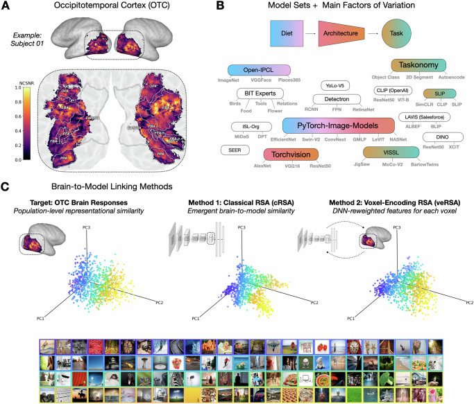
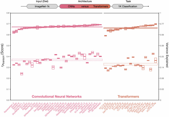
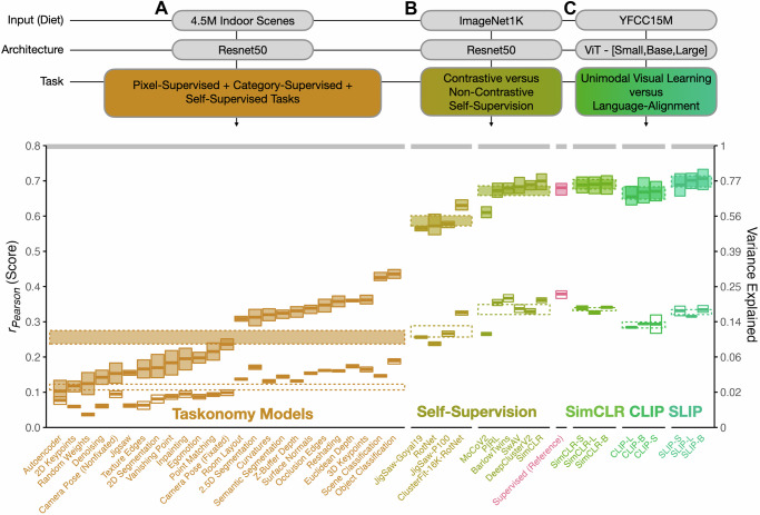
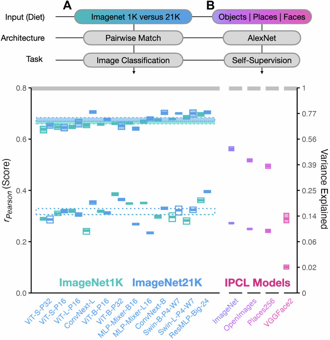
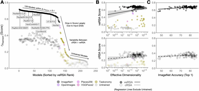
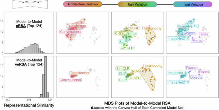
The rapid release of high-performing computer vision models offers new potential to study the impact of different inductive biases on the emergent brain alignment of learned representations. Here, we perform controlled comparisons among a curated set of 224 diverse models to test the impact of specific model properties on visual brain predictivity - a process requiring over 1.8 billion regressions and 50.3 thousand representational similarity analyses. We find that models with qualitatively different architectures (e.g. CNNs versus Transformers) and task objectives (e.g. purely visual contrastive learning versus vision- language alignment) achieve near equivalent brain predictivity, when other factors are held constant. Instead, variation across visual training diets yields the largest, most consistent effect on brain predictivity. Many models achieve similarly high brain predictivity, despite clear variation in their underlying representations - suggesting that standard methods used to link models to brains may be too flexible. Broadly, these findings challenge common assumptions about the factors underlying emergent brain alignment, and outline how we can leverage controlled model comparison to probe the common computational principles underlying biological and artificial visual systems.

Fig. 1. Overview of our approach.

A The brain region of focus is occipitotemporal cortex (OTC), here shown for an example subject. The voxel-wise noise-ceiling signal-to-noise ratio (NCSNR) is indicated in color. B A large set of models were gathered, schematized here by repository, and colored here by the main experiments to which they contribute. C Brain-linking methods. The left plot depicts the target representational geometry of OTC for 1000 COCO images, plotted along the first three principal components of the voxel space. Each dot reflects the encoding of a natural image, a subset of which are depicted below in a corresponding color outline. The middle panel shows a DNN representational geometry (here the final embedding of a CLIP-ResNet50), plotted along its top 3 principal components. Classical RSA involves directly estimating the emergent similarity between the brain target and the model layer representational geometries. The right plot shows the same DNN layer representation, but after the voxel-wise encoding procedure (veRSA), which involves first re-weighting the DNN features to maximize voxel-wise encoding accuracy, and then estimating the similarity between the target voxel representations and the model-predicted voxel representations. (Note: Images in C are copyright-free images gathered from Pixabay.com using query terms from the COCO captions for 100 of the original NSD1000 images. We are grateful to the original creators for the use of these images).

Fig. 2. Architecture variation.

Degree of brain predictivity (r_Pearson) is plotted for the controlled set of convolutional neural networks (CNNs) and transformer models in our survey. Each small box corresponds an individual model. The horizontal midline of each box indicates the mean score of each model’s most brain-predictive layer (selected by cross-validation) across the 4 subjects, with the height of the box indicating the grand-mean-centered 95% bootstrapped confidence intervals (CIs) of the model’s score across subjects. The cRSA score is plotted in open boxes, and the veRSA score is plotted in filled boxes. For each class of model architecture (convolutional, transformer) the class mean is plotted as a striped horizontal ribbon. The width of this ribbon reflects the 95% grand-mean-centered bootstrapped 95% CIs over the mean score for all models in a given set. The noise ceiling of the occipitotemporal brain data is plotted in the gray horizontal ribbon at the top of the plot, and reflects the mean of the noise ceilings computed for each individual subject. The secondary y-axis shows explainable variance explained (the squared model score, divided by the squared noise ceiling). Source data are provided as a Source Data file.

Fig. 3. Task variation.

Degree of brain predictivity (r_Pearson) is plotted for the sets of models with controlled variation in task. A The first set of models shows scores across the ResNet50 encoders from Taskonomy, trained on a custom dataset of 4.5 million indoor scenes. B The second set of models shows the difference between contrastive and non-contrastive self-supervised learning ResNet50 models (with a category-supervised ResNet50 for reference), trained on ImageNet1K. C The third set of models shows the scores across the vision-only and vision-language contrastive learning ViT-[Small,Base,Large] models from FaceBook’s SLIP Project, trained on the images (or image-text pairs) of YFCC15M. Each small box corresponds an individual model. In all subplots, the horizontal midline of each box indicates the mean score of each model’s most brain-predictive layer (selected by cross-validation) across the 4 subjects, with the height of the box indicating the grand-mean-centered 95% bootstrapped confidence intervals (CIs) of the model’s score across subjects. The cRSA score is plotted in open boxes, and the veRSA score is plotted in filled boxes. The class mean for each distinct set of models is plotted in striped horizontal ribbons across the individual models. The width of this ribbon reflects the 95% grand-mean-centered bootstrapped 95% CIs over the mean score for all models in this set. The noise ceiling of the occipitotemporal brain data is plotted in the gray horizontal ribbon at the top of the plot, and reflects the mean of the noise ceilings computed for each individual subject. The secondary y-axis shows explainable variance explained (the squared model score, divided by the squared noise ceiling). Source data are provided as a Source Data file.

Fig. 4. Input variation.

Degree of brain predictivity (r_Pearson) is plotted for the sets of models with controlled variation in input diet. A The first set of models shows scores across paired model architectures trained either on ImageNet1K or ImageNet21K (a ∼13× increase in number of training images). B The second set of models shows scores across 4 variants of a self-supervised IPCL-AlexNet model trained on different image datasets. Each small box corresponds an individual model. In all subplots, the horizontal midline of each box indicates the mean score of each model’s most brain-predictive layer (selected by cross-validation) across the 4 subjects, with the height of the box indicating the grand-mean-centered 95% bootstrapped confidence intervals (CIs) of the model’s score across subjects. The cRSA score is plotted in open boxes, and the veRSA score is plotted in filled boxes. The class mean for each distinct set of models is plotted in striped horizontal ribbons across the individual models. The width of this ribbon reflects the 95% grand-mean-centered bootstrapped 95% CIs over the mean score for all models in this set. The noise ceiling of the occipitotemporal brain data is plotted in the gray horizontal ribbon at the top of the plot, and reflects the mean of the noise ceilings computed for each individual subject. The secondary y-axis shows explainable variance explained (the squared model score, divided by the squared noise ceiling). Source data are provided as a Source Data file.

Fig. 5. Overall Model Variation.

A Brain predictivity is plotted for all models in this survey (N = 224), sorted by veRSA score. Each point is the score from the most brain-predictive layer (selected by cross-validation) of a single model, plotted for both cRSA (open) and veRSA (filled) metrics. Models trained on different image sets are labeled in color. B Brain predictivity is plotted as a function of the effective dimensionality of the most predictive layer, with veRSA scores in the top panel and cRSA scores in the bottom panel. The regression (± 95% CIs) line is fit only on trained variants of the models (excluding untrained variants). C Brain predictivity is plotted as a function of the top-1 ImageNet1K-categorization accuracy for the models (N = 108) whose metadata includes this measure (veRSA, top panel; cRSA bottom panel). The noise ceiling of the OTC brain data is shown as the gray horizontal bar at the top of each plot. Source data are provided as a Source Data file.

Fig. 6. Model-to-Model comparison.

Leftmost Panel: Histogram of the pairwise model-to-model representational similarity for the 124 highest-ranking trained models in our survey. The top panel indicates direct layer-to-layer comparisons, while the bottom panel reflects the feature-reweighted layer-to-layer comparisons. Rightward Panels: Results of a multidimensional scaling (MDS) analysis of the model-to-model comparisons, where models whose most brain-predictive layers (selected by cross-validation) share greater representational structure appear in closer proximity. The 3 plots in each row show datapoints output from the same MDS procedure (cRSA, top row; veRSA, bottom row), and the columns show different colored convex hulls that highlight the different model sets from the opportunistic experiments. Note the scale of the MDS plots is the same across all panels. NC-SSL and C-SSL correspond to Non-Contrastive and Contrastive Self-Supervised Learning, respectively. Objects, Faces, and Places correspond to the IPCL models trained on ImageNet1K / OpenImages, Places256, and VGGFace2, respectively. Source data are provided as a Source Data file.

References

1. DiCarlo, J. J., Zoccolan, D. & Rust, N. C. How Does the Brain Solve Visual Object Recognition? Neuron73, 415–434 (2012). - DOI - PMC - PubMed
1. Hubel, D. H., & Wiesel, T. N. Receptive fields and functional architecture of monkey striate cortex. J. Physiol.195, 215–243 (1968). - PMC - PubMed
1. Olshausen, B. A., Field, D. J. et al. Sparse coding of natural images produces localized, oriented, bandpass receptive fields. Submitted to Nature. Available electronically as ftp://redwood. psych. cornell. edu/pub/papers/sparse-coding. ps, 1995. Citeseer.
1. Krizhevsky, A., Sutskever, I. & Hinton, G. E. ImageNet classification with deep convolutional neural networks. In Advances in Neural Information Processing Systems, 1097–1105 (2012).
1. Yamins, D. L. et al. Performance-optimized hierarchical models predict neural responses in higher visual cortex. Proc. Natl Acad. Sci.111, 8619–8624, (2014). - PMC - PubMed
Publication types
LinkOut - more resources