An integrated view of the structure and function of the human 4D nucleome

Abstract

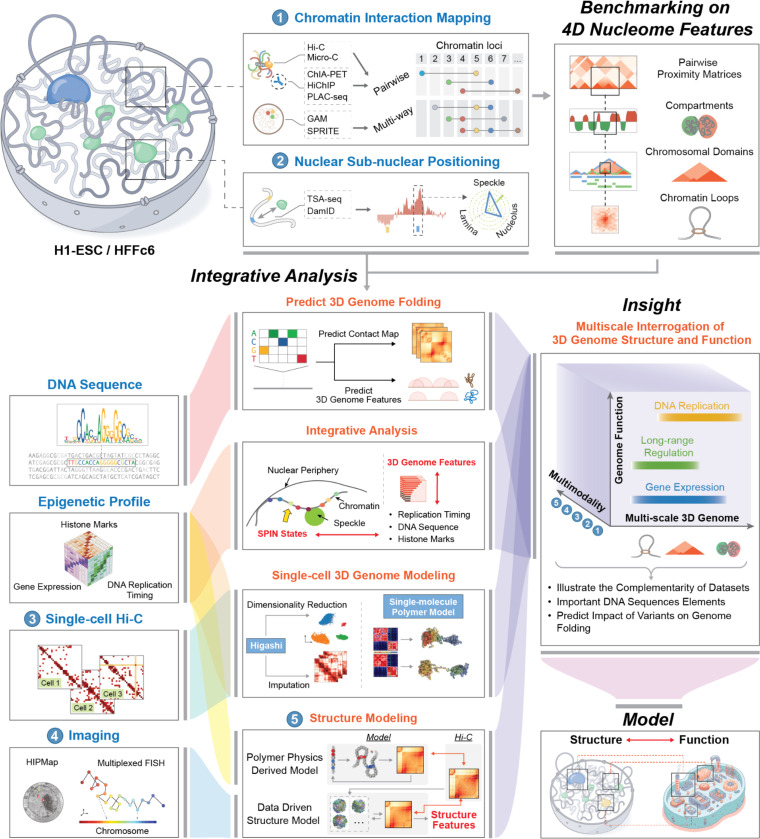
The dynamic three-dimensional (3D) organization of the human genome (the "4D Nucleome") is closely linked to genome function. Here, we integrate a wide variety of genomic data generated by the 4D Nucleome Project to provide a detailed view of human 3D genome organization in widely used embryonic stem cells (H1-hESCs) and immortalized fibroblasts (HFFc6). We provide extensive benchmarking of 3D genome mapping assays and integrate these diverse datasets to annotate spatial genomic features across scales. The data reveal a rich complexity of chromatin domains and their sub-nuclear positions, and over one hundred thousand structural loops and promoter-enhancer interactions. We developed 3D models of population-based and individual cell-to-cell variation in genome structure, establishing connections between chromosome folding, nuclear organization, chromatin looping, gene transcription, and DNA replication. We demonstrate the use of computational methods to predict genome folding from DNA sequence, uncovering potential effects of genetic variants on genome structure and function. Together, this comprehensive analysis contributes insights into human genome organization and enhances our understanding of connections between the regulation of genome function and 3D genome organization in general.

Extended Data Figure 1. Chromatin interaction assays quantitatively differ in detection of small compartment domains

a. Eigenvector 1 obtained from SPRITE data derived from a range of cluster sizes along a typical genomic loci, showing that small compartments are not detected when data from larger SPRITE clusters is used. b. Examples of Eigenvector 1 profiles obtained from data generated with the different genomic assays indicated. c. Compartmentalization strength calculated with interaction data obtained with different SPRITE clusters, for H1-hESC and HFFc6. e-f. Cumulative distributions of compartment sizes, as detected with Hi-C, Micro-C, ChIA PET, PLAC Seq, and SPRITE (cluster size 2–100) for H1-hESC and HFFc6 cells.

Extended Data Figure 2. Aggregate Peak Analysis for the same high-confidence chromatin loops in different platforms in H1-hESC (a) and HFFc6 (b).

The high-confidence loops for both cell lines were defined as those that can be identified by at least two methods. For each platform, distance-normalized signals at the 25 kb resolution within the 21×21pixel window centered at the coordinate of each loop are extracted and aggregated.

Extended Data Figure 3. Cross-platform loop comparisons in the HFFc6 cell line.

a. (top) Upset plot comparing loop anchors from different platforms. (bottom) Fold enrichment scores of ChromHMM states for each loop anchor category in the upset plot. b. UMAP projection and clustering of the 115,850 union loops in HFFc6 based on the composition of ChromHMM states at interacting loop anchors. c. For different loop clusters in panel b, we calculated fold enrichment scores of ChromHMM states, the median genomic distances between the loop anchors, and the average loop strengths in different platforms. SPRITE_2_10 represents a subset of DNA SPRITE clusters with 2–10 fragments. d. UMAP projection of chromatin loops from individual platforms.

Extended Data Figure 4. Transcription factor binding signatures of different loop clusters in H1-hESC.

a. ChIP-Seq binding profiles of selected transcription factors surrounding both anchors from different loop clusters. Each row represents one loop. b. Fraction of loop anchors bound versus fold enrichment for 62 transcription factors.

Extended Data Figure 5. 3D Structural features and their cell-to-cell variabilities in relation to gene function.

a. Distributions of speckle association frequencies (SAF) for chromatin in different SPIN states calculated from a population of 3D structures of HFFc6 genomes. b. tSNE projections of structure feature vectors for chromatin in different SPIN states in HFFc6. c. Distributions of SAF and normalized radial positions for chromatin in different SPIN states calculated from a population of 3D structures of H1-hESC genomes. d. Log-fold enrichment of 14 3D structural features for chromatin in different SPIN states calculated from the population of models. e. Distribution of speckle association frequencies for chromatin in different gene expression categories in HFFc6. f. Distribution of gene expression levels for housekeeping and non-housekeeping genes stratified by their speckle association frequencies. g. (left top panel) Distribution of gene expression levels taken from 6 gene expression experiments for POUF31 gene in H1-hESC and HFFc6. (second panel from right). 2D distribution of joint speckle distance and lamina distance for POU3F1 genes in 1000 single cell models. (right top panel) Schematic view of structural features in single cell models. RAD: radial position, LaD, Distance to the nuclear envelope, SpD: Distance to the closest speckle. (remaining panels) Cumulative distributions from single cell structure features of POU3F1 gene in the simulated cell population. (speckle distance, inter-chromosomal contact probability (ICP), transAB ratio). h. (left panel) Gene expression levels of THBS1 in H1-hESC and HFFc6 cells. (middle top panel) distribution of joint speckle distance and lamina distance for THBS1 genes in 1000 single cell models. (lower panels) log-fold enrichment of 14 structure features for THBS1 gene in H1ESC and HFFc6 cells. (Most Right panel), the same panels are shown also for the gene CAV1. i. (left panel) Gene expression levels of ACTB in H1ESC and HFFc6 cells. (Middle top panel) distribution of joint speckle distance and lamina distance for ACTB genes in 1,000 single cell models. (lower panels) Structure feature enrichment for ACTB gene in H1-hESC and HFFc6 cells. j. Scheme illustrating decreased contributions from long-range sequence distances for class I and increased contributions for class II genes.

Extended Data Figure 6. House-keeping genes are engaged in extensive enhancer-promoter loops.

For each boxplot, the center line indicates the median, the box limits represent the upper and lower quartiles, and the box whiskers extend to 1.5 times the interquartile range above and below the upper and lower quartiles, respectively. a. Size distributions of enhancer-promoter (EP) loops and CTCF-mediated loops. Data were merged from the H1-hESC and HFFc6 cells. b. Gene transcription levels versus the number of interacting enhancers in HFFc6. TPM, transcripts per kilobase million. c. Fold-change of gene transcription levels (TPM) is depicted for three gene groups: genes with a higher number of interacting enhancers in H1-hESC, genes with the same number of interacting enhancers in both cell lines, and genes with a higher number of interacting enhancers in HFFc6. The P values were computed using the two-sided Mann–Whitney U-test. d. Expression breadth of genes with different numbers of interacting enhancers in HFFc6. e, Distance-normalized contact signals between house-keeping gene promoters and regions (+/−30 kb) surrounding the interacting enhancers. f. Comparison of the number of interacting enhancers between the two house-keeping gene classes defined in the 3D modeling section. The P values were computed using the two-sided Mann–Whitney U-test. g. Expression breadth of genes with different number of interacting enhancers. Data were merged from 32 cell lines or primary cells. In each sample, genes are categorized into 11 groups based on the percentile of the number of interacting enhancers. h. Enrichment of house-keeping genes across gene sets characterized by the number of interacting enhancers and supported samples. Each bin represents a specific combination of these factors. For instance, the top-right corner bin represents the enrichment score for genes with the number of interacting enhancers greater than the 90th percentile across over 10 samples.

Extended Data Figure 7. Enhancer-promoter loops within nuclear lamina and their relationships with gene regulation.

For each boxplot, the center line indicates the median, the box limits represent the upper and lower quartiles, and the box whiskers extend to 1.5 times the interquartile range above and below the upper and lower quartiles, respectively. a-b. The distributions of the number of interacting enhancers for genes in different SPIN states in H1-hESC (a) and HFFc6 (b). c. Comparisons of transcription levels for genes with or without interacting enhancers in the Lamina SPIN state. The P values were calculated using the two-sided Mann-Whitney U test. d. Examples showing expressed genes, and their interacting enhancers are usually synergistically looped out of nuclear lamina to facilitate gene regulation in lamina. The blue arcs represent chromatin loops linking the gene in the center of each region with distal enhancers. e. Lamin-B1 DamID-seq signals surrounding lamina-associated genes and their interacting enhancers in HFFc6. Only genes with interacting enhancers in the Lamina SPIN state are included in this plot. TSS, transcription start sites. TES, transcription end sites. TPM, transcripts per kilobase million.

Extended Data Figure 8. Compartment and SPIN integration with replication timing, RNA-seq, and nascent transcripts from iMargi.

a, b. Averaged Hi-C, replication timing (16 fraction Repli-seq), nascent transcription (iMargi), and mRNA levels (RNA-seq) for h1ESCs at all A/B compartments (column 1) and SPIN states either co-registered or co-localized within A/B compartments (columns 2–10). All genomics data is plotted as the average signal across all genomic intervals representing SPINs in a particular column. SPIN genomic intervals of (SPIN genomic interval +/− flanks of 60% of the size of the genomic interval) are stretched laterally to scale by size before average signal is computed. a. All A compartments or select SPINS co-registered or within compartment A and b. All B compartments or select SPINS co-registered or within compartment B. Tracks show pileups in h1ESC for Hi-C Aggregate-Peak-Analysis (APA), A/B compartment, 16 fraction Repli-seq, median RNA-seq signal, condensed RNA-seq reads, median averaged iMARGI (+) and iMARGI (−) signal, condensed iMARGI (+) and iMARGI (−) reads, median iMARGI (+) signal, condensed iMARGI (+) reads, median iMARGI (−) signal, and condensed iMARGI (−) reads.

Extended Data Figure 9. Compartment, SPIN, and TAD integration with replication timing, RNA-seq, and nascent transcripts from iMargi.

a. Schematic depicting TAD (pink) and subTADs (blue) domains and loops (green circle). Dot domains contain a loop at the domain apex and dot boundaries. Dotless domains do not contain a loop at the apex and thus only dotless boundaries. b.,c. Dot and dotless TAD/subTAD domains that are within or co-register with a SPIN state contained within or co-registering with A/B compartments. b. Number of and c. proportion of SPINs stratified by A/B compartment and presence of corner-dot TAD/subTAD domains. d.-g. Averaged Hi-C, replication timing (16 fraction Repli-seq), mRNA levels (RNA-seq) for H1-hESCs at dot and dotless TAD/subTAD domains co-registered or co-localized within all SPIN states (columns 1–9) and TAD/subTAD domains with other SPIN alignment (column 10) either co-registered or co-localized within A/B compartments. All genomics data is plotted as the average signal across all genomic intervals representing domains in a particular column. TAD/subTAD genomic intervals of (TAD/subTAD genomic interval +/− flanks of 60% of the size of the genomic interval) are stretched laterally to scale by size before average signal is computed. d. Dot and e. dotless TAD/subTAD domain co-registered or within a SPIN and co-registered or within compartment A and f. Dot and g. dotless TAD/subTAD domain co-registered or within a SPIN and co-registered or within compartment B. Tracks show pileups in H1-hESC for Hi-C Aggregate-Peak-Analysis (APA), 16 fraction Repli-seq, median RNA-seq signal, condensed RNA-seq reads.

Extended Data Figure 10. Comparison of IZ properties across cell lines.

a.-c. Boxplots showing the minimum diamond insulation score at IZs in H1-hESC (a), HCT116 (b) and mESC (b). d.-f. Boxplots showing the total chromatin accessibility at IZs in H1-hESC (d), HCT116 (e), and mESC (f). g.-i. Boxplots showing the total RNA signal in H1-hESC (g), HCT116 (h), and mESC (i). j.-l. Average histone marks signal in 1Mb regions centered on IZs in H1-hESC (j), HCT116 (k), and mESC (l). Boxplots represent the median and interquartile range (IQR); whiskers mark 1.5x the IQR; data beyond 1.5x the IQR are plotted as individual points.

Figure 1

Overview of the key highlights from the first phase of 4D Nucleome project. (Top-left) Schematic plots illustrate two types of complementary genomic assays for mapping 3D genome folding and the relative distances of genomic loci to nuclear bodies in H1-hESC and HFFc6 cells. (Top-right) Different chromatin interaction mapping methods are compared and benchmarked to assess their ability to identify and quantify 3D genome features at scales ranging from chromatin compartments (Mb) to focally enriched chromatin interactions (kb). (Bottom-left) Additional multimodal datasets generated or utilized to facilitate integrative analyses (see below). (Bottom-center) Multiple integrative modeling and analysis approaches are conducted to reveal the spatial features of chromatin loci by combining 3D genome features and various multimodal datasets. The connections between different input data and integrative analyses is illustrated through color-coded flow paths. (Bottom-right) An illustrative cartoon summarizes the overarching aim of the project: to provide novel insights into structure-function relationships by connecting variable 3D genome features (represented on the X-axis) derived from multimodal datasets (Y-axis) with key cellular functions, such as transcription and replication (Z-axis). Our models are paving the way for identifying the sequence determinants of genome folding and predicting how different variants might influence this folding process.

Figure 2. Methods for chromatin interaction detection differ in quantitative detection of compartmentalization

a. (Upper panel) Heatmaps of contact maps generated using Hi-C, Micro-C, ChIA-PET, PLAC-Seq, and SPRITE (100 kb bins, chr. 2 0–70 Mb) derived from HFFc6 cells. (Lower Panel) Zoomed heatmaps of contact maps (25 kb bins, chr2 12–16mb) b. Spearman correlation of compartment profiles determined by Eigenvector decomposition (see Supplemental Methods). c. Compartment strength quantified using eigenvectors detected and quantified from contact data obtained with corresponding 3D methods d. Pearson correlation of genome-wide insulation scores for all methods. e. Aggregated insulation scores at strong boundaries detected in multiple datasets (see Supplemental Methods), using data obtained from indicated methods. f. Preferential interactions quantified in Hi-C, Micro-C, ChIA-PET, PLAC Seq, SPRITE and GAM, using DamID Seq for Lamin B, Early and Late replication timing (E/L RT) using RepliSeq, and TSA Seq for SON to rank loci: The fold enrichment indicates the preference of loci with similar associations with speckles (SON), nucleoli (PolR1E/NFIK), lamina (Lamin B), or that display early or late replication to interact with each other, as detected by the indicated interaction assays.

Figure 3. Cross-platform loop comparisons.

We identified and compared chromatin loops from 5 experimental methods: Hi-C, Micro-C, CTCF ChIA-PET, RNA Pol II ChIA-PET, and H3K4me3 PLAC-Seq. a. The number of detected loops in each platform in two 4DN tier 1 cell lines H1-hESC and HFFc6. In panels b-g, we only included data from H1-ESC. b. (top) Upset plot comparing loop anchors from different platforms. (bottom) Fold enrichment scores of ChromHMM states for each loop anchor category in the upset plot. The bar plot on the right represents the number of loop anchors overlapping with different chromatin states, and different colors in a bar represent different categories in the upset plot. c. UMAP projection and clustering of the 124,061 union loops in H1-ESC based on the composition of ChromHMM states at interacting loop anchors. d. For different loop clusters in panel c, we calculated fold enrichment scores of ChromHMM states, the median genomic distances between the loop anchors, and the average loop strengths in different platforms. SPRITE_2_10 represents a subset of DNA SPRITE clusters with 2–10 fragments. e. UMAP projection of chromatin loops from individual platforms. f. An example showing the differences of platforms in detecting insulator-related loops. Contact maps are plotted at the 5 kb resolution, and chromatin loops are marked by blue circles. g. An example showing the differences of platforms in detecting transcription-related loops. Contact maps are plotted at the 1kb resolution, and chromatin loops are marked by blue circles.

Figure 4. SPIN states stratify the genome into distinct spatial compartments.

Heatmaps show the enrichment of histone marks, Repli-seq signals, and caRNAs (columns) on different SPIN states (rows). Colors of the heatmap indicate the log2 fold-change enrichment calculated as the ratio of observed signals over genome-wide expectation.

Figure 5. 3D Structural features and their cell-to-cell variabilities in relation to gene function.

a. Single cell genome structure model of the H1-hESC with genomic regions color coded by their SPIN states. b. Slice through genome structure in A with only a few chromosomes shown together with predicted speckle locations by red spheres, c. Enrichment of different structural features for chromatin in different SPIN states calculated from the population of models. RAD: 1-norm. average radial position, RG: chromatin fiber de-compactness (radius of gyration of chromatin fiber over +/−500kb), SpD: average speckle distance, NuD: average distance to nucleolus, ILF: interior localization probability (fraction of alleles within 50% percentile interior volume), SAF: speckle association frequency, LAF: lamina association frequency, ICP: inter chromosomal interaction probability, TransAB: trans A/B ratio, δ features (RAD, RG, Spd, Nud) show cell-to-cell variability of the respective feature (Methods). d. Box plots for the distributions of average radial positions of chromatin regions in each SPIN state e. Violin plots for distributions of speckle distance z-score differences for genes in H1-hESC and HFFc6 that are significantly up-regulated (up to 9-fold) and significantly down-regulated (by more than 9-fold) in HFF over H1. Shown are Z-score differences in speckle distances of genomic regions between both cell types (HFF - H1). f. Average radial positions for a part of chromosome 1 in H1-hESC cells (upper panel) and HFFc6 cells (lower panel). g. Log-fold enrichment of 14 structural features calculated for the POU3F1 gene in H1-hESC (upper panel) and HFFc6 cells (lower panel), calculated from the 3D structure population. h. (Left panel) Chromosome 1 in single cell 3D genome structure of H1-hESC (left panel) and HFFc6 (right panel). The nuclear location of POU3F1 gene is shown by a yellow circle, red color shows chromosomal regions annotated in the SPIN speckle state, blue regions show chromatin in the lamin SPIN state. Locations of predicted nuclear speckle locations closest to POU3F1 are shown. i. t-SNE projections of 3D structure feature vectors for chromatin regions containing the transcription start sites of genes with the highest and lowest expression quartiles in HFFc6, as well as chromatin regions without known genes. Shown are also the number of all genes in each group, while the number of housekeeping genes within each group are shown in parenthesis. j. t-SNE projections of the 25% most highly expressed genes with the top (left panel) and lowest SAF quartile among all genes (bottom panel). k. log-fold enrichment of 14 3D structure features for highly expressed genes (top quartile), lowly expressed genes (bottom quartile) genes in class I and class II microenvironments. l. log-fold enrichment for genomic properties (within a 200kb region), histone modifications (within +/− 10kb of TSS), and 3D spatial enhancer densities at each TSS (Methods) for highly expressed genes (top quartile), lowly expressed (bottom quartile) genes in class I and class II microenvironments. m. Comparison of the intrachromosomal 3D spatial enhancer density at TSS of housekeeping genes in class I (high SAF) and class II (low SAF) microenvironments. Only enhancers at a sequence distance >1Mb are considered.

Figure 6. Cell-to-cell variabilities of 3D genome features.

a. Heatmap on the top shows the merged scHi-C contact maps at a 2Mb region from chr3 imputed by Higashi (bottom-left) or predicted by the SBS polymer model (top-right). Insulation scores from bulk Hi-C, calculated insulation scores after Higashi imputation and SBS polymer modeling are shown at the bottom. b. 3D genome structure models, raw scHi-C contact cap, and the imputed contact map from three mutually similar cells between Higashi imputation and SBS model are shown. c. The average normalized intensity of chromatin loop across 188 WTC-11 cells is calculated and compared by dividing loops based on their relative position within TADs and A/B compartments. The pink boxplot (left) represents the difference between loops in the same TAD and loops spanning multiple TADs. The blue boxplot (right) shows the difference between loops in the same A/B compartment and loops spanning different compartments. A representative chromatin loop near gene RABGAP1L is highlighted in the box plot on the right. The original distribution of the normalized intensity of this specific loop in each cell is shown in the box plots on the right. Loops are stratified into different groups depending on whether this loop locates within one TAD or spans TADs (top) or the A/B compartments state of two loop anchors in each single cell.

Figure 7. Associations of enhancer-promoter loops with gene regulation.

a. Gene transcription levels versus the number of interacting enhancers in H1-hESC. For each boxplot, the center line indicates the median, the box limits represent the upper and lower quartiles, and the box whiskers extend to 1.5 times the interquartile range above and below the upper and lower quartiles, respectively. TPM, transcripts per kilobase million. b. Expression breadth (number of tissues a gene is expressed in) of genes with different number of interacting enhancers in H1-hESC. c. Percentages of house-keeping genes with different number of interacting enhancers. d. Genome browser view of a region surrounding the house-keeping gene EIF1. The blue arcs represent chromatin loops linking the EIF1 gene promoter with distal enhancers. e. The dynamics of chromatin loops linking house-keeping gene promoters and distal enhancers between H1-hESC and HFFc6. f. Genome browser view of the CMAS loci in H1-hESC. g. Lamin-B1 DamID-seq signals surrounding lamina-associated genes and their interacting enhancers in H1-hESC. Only genes with interacting enhancers in the Lamina SPIN state are included in this plot. TSS, transcription start sites. TES, transcription end sites. TPM, transcripts per kilobase million.

Figure 8. A/B compartments and SPIN states represent subnuclear regions of distinct replication timing and gene expression.

a. Schematic of human genome folding into A/B compartments, SPIN states, TADs, subTADs, and loops integrated with early/late replication timing and initiation zones. b. Intersection of SPIN states with compartments. SPIN states were classified as either fully embedded within A/B compartments (within), co-registering A/B compartments (co-register), or partially-overlapping (other) c. Fraction of each SPIN state co-registered or nested within A/B compartments in H1-hESCs. d,e. Averaged Hi-C, replication timing (16 fraction Repli-seq), nascent transcription (iMargi), and total mRNA (RNA-seq) signal is plotted for h1ESCs at all A/B compartments (column 1) or co-registered/nested within selected SPIN states in A/B compartments (columns 2–6). Data is plotted as the average signal across SPIN states. The genomic intervals representing SPINs +/− flanks of 60% of the SPIN size are stretched laterally to scale by size. d. All A compartments or selected SPINS co-registered/within compartment A. e. All B compartments or selected SPINS co-registered/within compartment B. f. Average chromatin landscape at IZs in H1ESC. IZs have been grouped depending on their replication timing (RT). Tracks represent the high-resolution replication timing, chromatin compartments, expression and histone marks. g. We computed right-tailed, one-tailed empirical p-values using a resampling test with size and A/B compartment-matched null IZs for the intersection of Early and Late S phase IZs with dot boundaries, dotless boundaries, and no boundaries. h. Example of chromatin profiles around IZs (portion of chr2 from 20Mb to 58Mb). Tracks represents the chromatin contacts, 4 groups of IZs depending on their RT, the high-resolution replication timing, chromatin compartments, the SPIN states, Expression (minus and plus strands), H3K27Ac, H3K4me3 and H2AX.

Figure 9. Predicting the effect of genomic variants on 3D genome folding with deep learning.

a. Example of a 345 bp deletion (chr1: 47262830–47263175) at the TAL1 locus. Contact maps (log(observed/expected)) were predicted for ~1Mb regions with a model trained on HFFc6 Micro-C data using the Akita architecture . Maps for the reference human genome sequence (WT) and the in silico mutated sequence (Mut; at center) are plotted on a color scale where red indicates higher than expected interaction frequencies, and blue indicates lower than expected given genomic distance. The effect of the deletion (Mut - WT) is plotted on a color scale where purple indicates increased and green decreased chromatin interactions. Genes in the locus are plotted below the contact maps with TAL1 highlighted in red. The deleted region has a CTCF binding site and is located in a TAD boundary. Mirroring the experimental deletion in HEK293T cells (Hnisz et al., 2016), our model predicted increased contact frequency between TAL1 and adjacent regions (black rectangle). b. In silico mutation of transcription factor motifs (replacing motifs with random sequences) affects deep learning predictions of nearby chromatin interactions. An example POU2F1::SOX2 motif (left, chr13: 81872756–81872772) and FOSL1::JUND motif (right, chr16: 12340569–12340578) were generated using models with the Akita architecture trained on H1-hESC or HFFc6 Micro-C data, respectively. Motif logos generated via model importance scores using DeepExplainer are shown below the maps. Color scales are the same as in (a), and motif sites are centered on the contact maps. Star symbols indicate regions with altered chromatin interaction predictions.

References

1. ENCODE-Project-Consortium. An integrated encyclopedia of DNA elements in the human genome. Nature 489, 57–74 (2012). - PMC - PubMed
1. Consortium, E. P. et al. Expanded encyclopaedias of DNA elements in the human and mouse genomes. Nature 583, 699–710 (2020). 10.1038/s41586-020-2493-4 - DOI - PMC - PubMed
1. Furlong E. E. M. & Levine M. Developmental enhancers and chromosome topology. Science 361, 1341–1345 (2018). 10.1126/science.aau0320 - DOI - PMC - PubMed
1. Robson M. I., Ringel A. R. & Mundlos S. Regulatory Landscaping: How Enhancer-Promoter Communication Is Sculpted in 3D. Mol Cell 74, 1110–1122 (2019). 10.1016/j.molcel.2019.05.032 - DOI - PubMed
1. Galouzis C. C. & Furlong E. E. M. Regulating specificity in enhancer-promoter communication. Curr Opin Cell Biol 75, 102065 (2022). 10.1016/j.ceb.2022.01.010 - DOI - PubMed
Publication types
LinkOut - more resources