Topography of putative bidirectional interaction between hippocampal sharp wave ripples and neocortical slow oscillations

Abstract

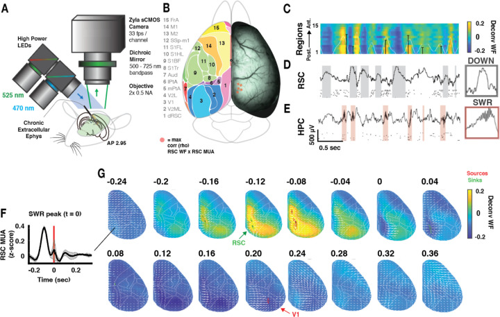
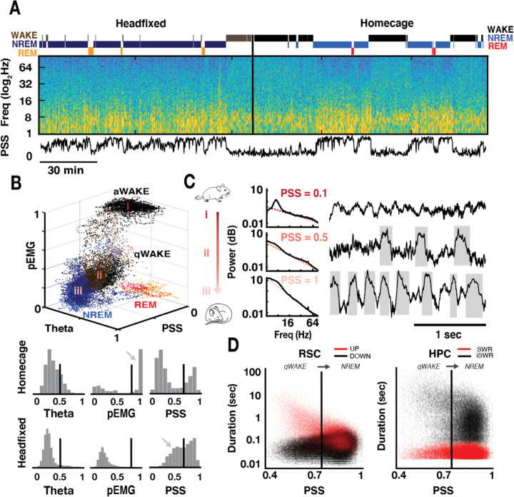
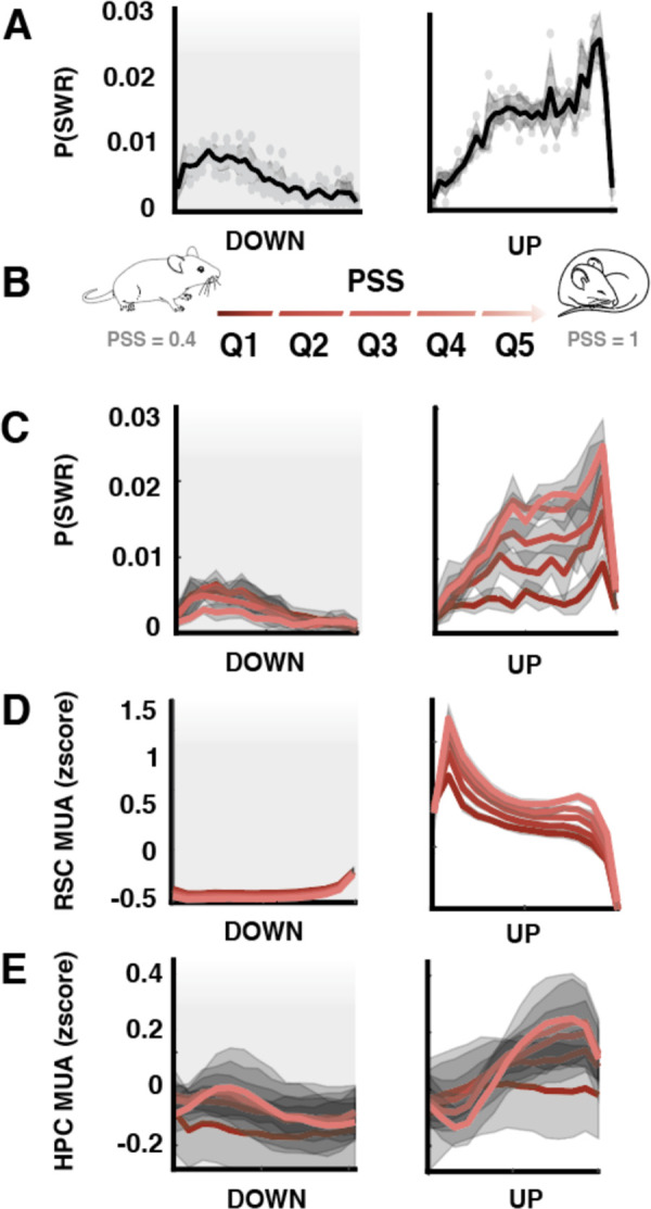
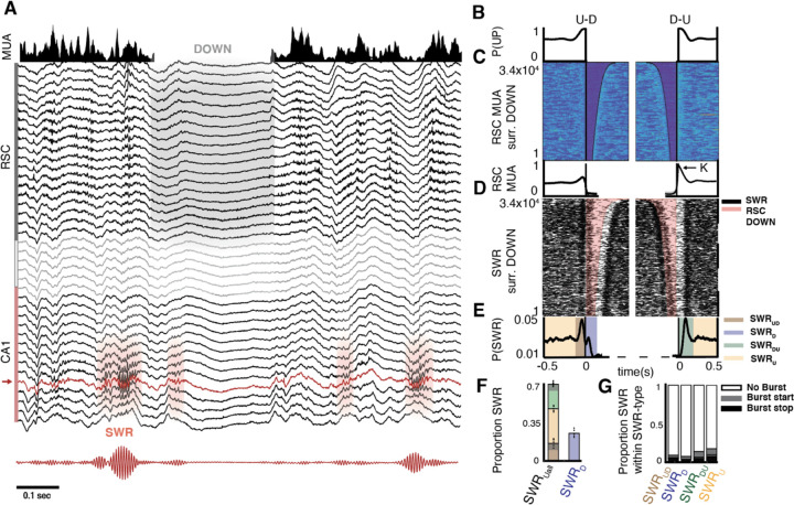
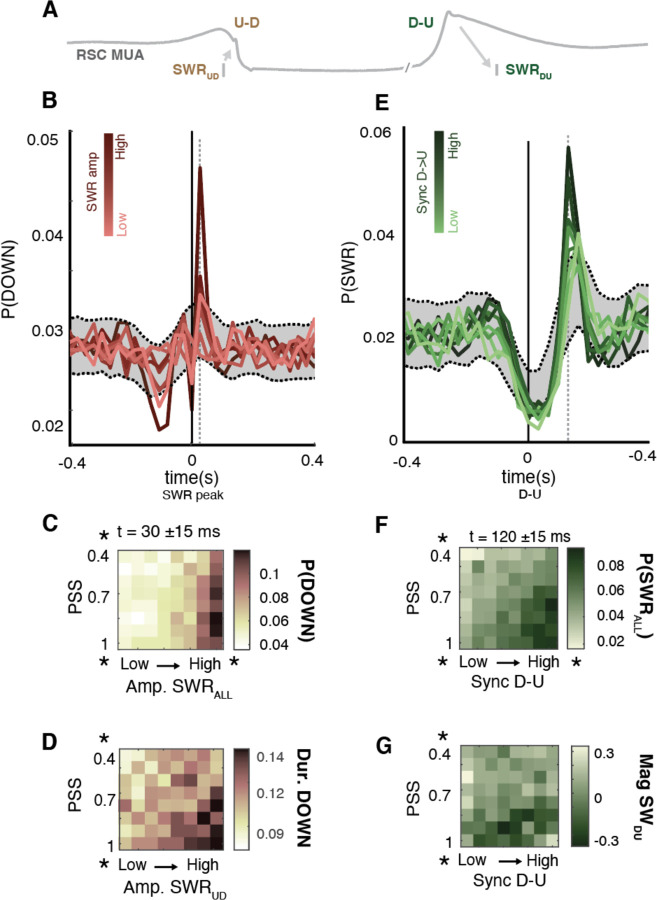
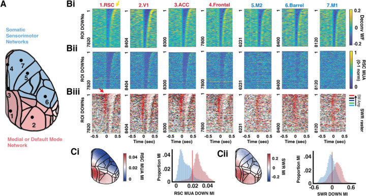
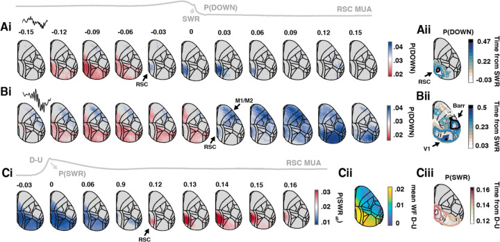
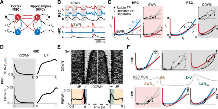
Systems consolidation relies on coordination between hippocampal sharp-wave ripples (SWRs) and neocortical UP/DOWN states during sleep. However, whether this coupling exists across neocortex and the mechanisms enabling it remain unknown. By combining electrophysiology in mouse hippocampus (HPC) and retrosplenial cortex (RSC) with widefield imaging of dorsal neocortex, we found spatially and temporally precise bidirectional hippocampo-neocortical interaction. HPC multi-unit activity and SWR probability was correlated with UP/DOWN states in mouse default mode network, with highest modulation by RSC in deep sleep. Further, some SWRs were preceded by the high rebound excitation accompanying DMN DOWN→UP transitions, while large-amplitude SWRs were often followed by DOWN states originating in RSC. We explain these electrophysiological results with a model in which HPC and RSC are weakly coupled excitable systems capable of bi-directional perturbation and suggest RSC may act as a gateway through which SWRs can perturb downstream cortical regions via cortico-cortical propagation of DOWN states.

Figure 1.. Experimental preparation and neocortical activity surrounding hippocampal SWRs.

A. Dual wavelength (blue 470 nm – thy1 GCaMP6f; green 525 nm – total blood volume) widefield imaging (66 frames per second) of the dorsal hemisphere of a thy1 GCaMP6f mouse. Note chronic silicon probe spanning ipsilateral CA1 and RSC beneath the imaging field of view (green). B. Right, Example raw fluorescence frame. Left, Corresponding cortical regions. Red dots indicate location of maximum correlation (rho) between widefield signal and RSC population rate for each mouse (n=5). C-E. Aligned simultaneous widefield imaging of dorsal cortex and electrophysiological recordings in HPC and RSC. C. Deconvolved widefield time series for 15 pixels in regions ranging from posterior to anterior dorsal cortex as in B. White line corresponds to RSC widefield time series (also row 1 in heat map); black bars denote SWRs, height proportional to SWR amplitude. D-E. Example LFP and single units from RSC and hippocampal CA1 pyramidal layer. Shaded areas highlight DOWN states and SWRs in RSC and HPC, respectively. Right insets, example DOWN state and SWR (100 ms). F. Average RSC multi-unit activity (MUA; see Methods) surrounding all SWR peaks at t = 0. Shading corresponds to standard deviation across mice (n = 5). G. Average deconvolved widefield activity across all mice surrounding SWR peak at t = 0. Sources and sinks are identified in green and red, respectively. Arrows correspond to vector fields calculated across pairs of frames on the grand-average video, providing a qualitative view of activity flow.

Figure 2.. SWR and DOWN state rates increase as animals move from quiet wake to deep NREM sleep.

A. Brain state-scoring of concatenated headfixed and home cage recording sessions for an example mouse. Top, Identified WAKE, NREM, and REM states. Middle, spectrogram of RSC LFP. Bottom, Time-varying slope of the power spectrum (PSS). B. Top, State scoring of the session in panel A. Note three distinct clusters, classified as active wake (aWAKE), REM sleep, and a third cluster with continuous variation from quiet wake (qWAKE) to NREM sleep. Bottom, Distributions of the three variables used for behavioral state scoring (PSS, proxy EMG, and theta power) in homecage and headfixed conditions. C. Average RSC power spectra (black; left) and example RSC LFP traces (right) at three different arousal levels from active WAKE to deep NREM, denoted i-iii in panel B scatterplot. Inset PSS values are the inverse of the slope of the linear fit to the aperiodic component of the power spectra (pink dotted lines). DOWN states are shaded in gray. D. Left, Scatter plot of durations of UP (red) and DOWN (black) states in RSC across values of PSS for all mice. Right, Scatter plot of dwell time durations for SWRs (red) and inter-SWR periods (black). Vertical lines in RSC and HPC separate qWAKE and NREM.

Figure 3.. RSC UP and DOWN states modulate hippocampal SWRs as a function of brain state.

A. Probability of SWRs across time-normalized RSC UP and DOWN states. Shading corresponds to standard deviation across mice; dots to individual mice. B. PSS quintiles span quiet WAKE to deep NREM (Q1-Q5; colored from dark to light red in all panels). C-E. Variables specified plotted across time-normalized RSC UP and DOWN states as a function of PSS quintile; all mice. Shading corresponds to standard deviation across all UP or all DOWN states. C. Probability SWR by PSS quintile. D. Mean RSC MUA by PSS quintile. E. Mean HPC MUA by PSS quintile.

Fig 4.. Probability of SWRs around UP-DOWN (U-D) and DOWN-UP (D-U) transitions is asymmetric.

A. Example LFP traces spanning layers of granular RSC, white matter, and ipsilateral CA1; RSC MUA (above); ripple frequency filtered CA1 trace (below; 130–200 Hz; bandpass filtered channel designated in red). B-E. Data specified surrounding all DOWN states for an example mouse, centered at RSC U-D transitions (left) or D-U transitions (right) and sorted by DOWN state duration. B. Probability of being in an UP state, surrounding transitions. C. RSC MUA; each row is an U-D (left) or D-U (right) transition (>30,000). Bottom, average RSC MUA surrounding transition specified. K refers to transient rebound population synchrony at the D-U transition, K-complex or ‘K’. D. Raster plot of all SWRs during the same RSC U-D and D-U transitions as in C. Pink shading corresponds to RSC DOWN states identified in panel C. SWRs plotted as thin black lines, the length of which corresponds to their durations. Note decreased P(SWR) during DOWN, asymmetry in clustering of SWRs around transitions, and change in clustering as DOWN duration increases. E. Defining SWRs by their temporal proximity to U-D and D-U transitions yields 4 “types”, SWR_U (yellow), SWR _UD (red), SWR D (blue), and SWR DU (green); see Methods and Fig. S6. F. Proportion of each “SWR type” across all mice (dots represent individual mice; colors correspond to SWR type). Note 3-fold increase in SWR rate from DOWN to UP states. Gray shaded region in SWR_UD and SWR_DU represents the overlap between these categories (~30%). G. For each SWR type, proportion of those SWRs that occur in bursts vs not in bursts (see Methods). Start and end times of the burst are denoted by gray and black.

Figure 5.. Temporal relationship between HPC and RSC state transitions is state-dependent and bi-directional

A. Schematic of hypothesis: SWRs can induce U-D transitions and D-U transitions can induce SWRs, conditional on magnitude of the perturbation and state of the receiving region. B. Cross-correlograms between SWR peaks (t = 0 s) and DOWN state onsets across all mice, colored by SWR amplitude octile (light to dark red; small to large SWRs). Shading denotes boot-strapped 99% confidence intervals obtained by shuffling both SWRALL peak and U-D time series by ±30ms, 1000 iterations. Note increased probability of DOWN onset at fixed 30 ± 15 ms timelag (vertical gray line) with increasing SWR amplitude. C. Mean probability of DOWN state onset at a 30ms lag from SWR peak, timelag of putative ‘interaction’, as a function of depth sleep (PSS) and SWRALL amplitude (repeated measures two-way ANOVA across sessions (n=15): R2 = 0.47. SWR amplitude, F = 83.19, p < 0.001, η^²p = 0.42; PSS, F = 5.87, p < 0.001, η^²p = 0.07; Interaction, F = 1.68, p < 0.05, η^²p = 0.06). Significant effect of amplitude SWR, depth sleep, and their interaction. D. Mean duration of DOWN states following SWR_UD as a function of depth sleep (PSS) and SWR_UD amplitude across all mice (GLM 5-fold CV: R2 = 0.014. SWR amplitude β1 = −0.007, t = 0.006, p = NS; PSS β1 = 0.067, t = 7.68, p < 0.001; Interaction β1 = −0.016, t = 1.96, p < 0.05). E. Probability of SWRs surrounding RSC D-U transitions (t = 0s), colored by D-U rebound excitation octile (light to dark green, small to large). Note increase in P(SWR) with increasing rebound excitation at a fixed lag of 120ms (vertical gray line). Confidence intervals computed as in B. F. Mean probability of SWR occurrence at a 120ms lag from RSC D-U as a function of depth sleep (PSS) and D-U rebound excitation (repeated measures two-way ANOVA: R2 = 0.58. Rebound excitation, F = 54.01, p < 0.001, η^²p = 0.32; PSS, F = 120.26, p < 0.001, η^²p = 0.42; Interaction, F = 3.78, p < 0.001, η^²p = 0.15. K. Mean magnitude of HPC sharp-waves as a function of tonic MUA HPC and D-U rebound excitation across all mice (GLM 5-fold CV: R2 = 0.05. Rebound excitation β1 = −0.27, t = −1.65 p = NS; PSS β1 = −1.01, t = −5.02, p < 0.001; Interaction β1 = 0.4, t = 1.95, p < 0.05).

Figure 6.. Probability of SWRs surrounding DOWN states across dorsal neocortex.

A. Map of regions visible in imaging FOV, color-coded by membership in medial network (red) or somatic sensorimotor networks (blue), as in [39]. Numbered regions correspond to columns in Bi-iii. Bi. Deconvolved widefield activity surrounding widefield-detected DOWN states in the region specified (25^th percentile of pixel WF values and below = DOWN state), as described in Fig. S8 and Methods. Sorted by duration DOWN for an example mouse, separately in each region. Bii. RSC MUA surrounding the same DOWN states for each region. Biii. Raster plot of SWRs surrounding the same DOWN states, color-coded by SWR amplitude quintiles (small to large: green, cyan, blue, black, red). Note that large amplitude SWRs (red) precede U-D transitions for long DOWN states, red arrow. Ci. Average modulation index (MI; see Methods) of RSC MUA by DOWN states detected across all pixels and all mice; positive MI corresponds to higher RSC MUA during UP than DOWN for the given pixel (see Methods for details); Left, MI plotted on dorsal map, Right, distribution of same values separated by medial (red) and sensorimotor networks (blue). Cii. Average modulation of SWRs by DOWN states across all regions; Left, MI plotted on dorsal map, Right, distribution of same values separated by medial (red) and sensorimotor networks (blue).

Figure 7.. Average topography of putative interaction between hippocampal SWRs and neocortical DOWN states. Ai.

Average probability of DOWN state occurrence across all pixels aligned to low amplitude SWRs (amplitude quintile 1 of 5; t = 0, peak of SWRs). Colored portion of plots denotes the timepoints at which the given pixel is above (blue) or below (red) a 95^th percentile bootstrapped confidence interval, obtained by shuffling SWR peak times across all SWRs and re-computing cross correlograms (n=500). Aii. Outline of DOWN states from the onset of DOWN in RSC (white outline) to a sink in RSC (dark blue outline), colored by latency with respect to SWR peak. Bi. Same as Ai but for SWR amplitude quintile 5 of 5. Note onset of DOWN states 30 ms following SWR peak in both RSC and regions across sensorimotor network. Bii. Outline of DOWN states from onset of DOWN in RSC and sensorimotor regions (white outlines) to sinks in V1 and barrel cortex (dark blue outlines), colored by latency with respect to SWR peak. Ci. The probability of SWR occurrence aligned to D-U transitions (t = 0) for every pixel. Colored portion of plots denotes the timepoints at which the given pixel is above (blue) or below (red) a 95^th percentile bootstrapped confidence interval, computed as in Ai and Bi but with shuffled D-U transition times. Cii. Mean widefield activity within 20 ms of the D-U transition for each pixel. Ciii. Outline of significant increase in P(SWR) following D-U transitions for successive frames.

Figure 8.. Model of the bidirectional interactions between Hippocampus and Retrosplenial Cortex.

A. Two-region firing rate model of HPC and RSC with long-range projections between the two regions. Each region comprises of recurrently connected Excitatory (E) and Inhibitory (I) populations with independent background noise. The E populations are subject to a slow feedback current (h-current (h) in RSC, adaptation (a) in HPC, see Methods). B. Model simulation outputs for E and I populations in the two regions, and feedback currents. C. I-E phase planes for RSC and HPC. Both regions show two stable steady states (a DOWN and an UP state for RSC and an iSWR and a SWR state for HPC). The basin of attraction for each steady state is bounded by a separatrix passing through an unstable fixed point (FP). In the hippocampus (left), a transition from the iSWR to the SWR state engages the adaptative current, which destabilizes the SWR state. In the cortex (right), a transition from the UP to the DOWN state engages the h-current, which destabilizes the DOWN state. D. From top to bottom: HPC MUA and P(SWR) plotted as a function of time-normalized RSC UP and preceding DOWN states (compare to Fig. 3). E. Top. Raster plot of all SWRs surrounding the DOWN state. Note as in experimental data, clustering of SWRs around UP and DOWN state transitions. Bottom. P(SWR) surrounding state transitions reveal a peak before the U-D transition and after the D-U transition (compare to Fig. 4). F. Analysis of the phase planes for SWR-UP/DOWN interaction. (i, SWR_UD) Increased hippocampal activity in the SWR state displaces the RSC nullclines, destabilizing the UP state fixed point and pushing the trajectory to a DOWN state. (ii) Low RSC activity in the DOWN state lowers the HPC E nullcline, reducing the P(SWR). (iii, SWR_DU) Activation of the h-current during the DOWN state results in increased RSC activity following the D-U transition. High RSC activity displaces the HPC nullclines, destabilizing the iSWR fixed point and pushing the trajectory to a SWR.

References

1. McClelland J. L., McNaughton B. L., and O’Reilly R. C., “Why there are complementary learning systems in the hippocampus and neocortex: insights from the successes and failures of connectionist models of learning and memory.,” Psychol. Rev., vol. 102, no. 3, pp. 419–457, 1995, doi: 10.1037/0033-295X.102.3.419. - DOI - PubMed
1. Kumaran D., Hassabis D., and McClelland J. L., “What Learning Systems do Intelligent Agents Need? Complementary Learning Systems Theory Updated,” Trends in Cognitive Sciences, vol. 20, no. 7. Elsevier Ltd, pp. 512–534, 2016, doi: 10.1016/j.tics.2016.05.004. - DOI - PubMed
1. Alvarez P. and Squire L. R., “Memory consolidation and the medial temporal lobe: A simple network model,” Proc. Natl. Acad. Sci. U. S. A., vol. 91, no. 15, pp. 7041–7045, 1994, doi: 10.1073/pnas.91.15.7041. - DOI - PMC - PubMed
1. Buzsáki G., “Hippocampal sharp wave-ripple: A cognitive biomarker for episodic memory and planning,” Hippocampus, vol. 25, no. 10, pp. 1073–1188, 2015. - PMC - PubMed
1. Wittkuhn L., Chien S., Hall-McMaster S., and Schuck N. W., “Replay in minds and machines,” Neurosci. Biobehav. Rev., vol. 129, no. August, pp. 367–388, 2021, doi: 10.1016/j.neubiorev.2021.08.002. - DOI - PubMed
Publication types
LinkOut - more resources