Deciphering the topological landscape of glioma using a network theory framework

Abstract

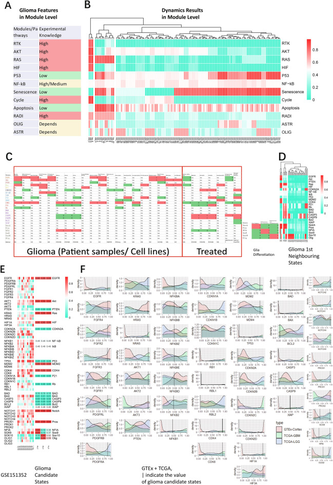
Glioma stem cells have been recognized as key players in glioma recurrence and therapeutic resistance, presenting a promising target for novel treatments. However, the limited understanding of the role glioma stem cells play in the glioma hierarchy has drawn controversy and hindered research translation into therapies. Despite significant advances in our understanding of gene regulatory networks, the dynamics of these networks and their implications for glioma remain elusive. This study employs a systemic theoretical perspective to integrate experimental knowledge into a core endogenous network model for glioma, thereby elucidating its energy landscape through network dynamics computation. The model identifies two stable states corresponding to astrocytic-like and oligodendrocytic-like tumor cells, connected by a transition state with the feature of high stemness, which serves as one of the energy barriers between astrocytic-like and oligodendrocytic-like states, indicating the instability of glioma stem cells in vivo. We also obtained various stable states further supporting glioma's multicellular origins and uncovered a group of transition states that could potentially induce tumor heterogeneity and therapeutic resistance. This research proposes that the transition states linking both glioma stable states are central to glioma heterogeneity and therapy resistance. Our approach may contribute to the advancement of glioma therapy by offering a novel perspective on the complex landscape of glioma biology.

Keywords: Endogenous network theory; Energy landscape; Gene regulatory network; Glioma; Glioma stem cell; Network dynamics.

Fig. 1

Endogenous network and network dynamics frameworks for glioma. (A) The core endogenous network for glioma. This network, constructed from experimentally driven causality knowledge, comprises 10 core functional modules or molecular pathways, including the RTK pathway, NF-κB pathway, Ras pathway, Akt pathway, HIF pathway, p53 pathway, cell cycle, cellular senescence, apoptosis, and glia differentiation. A closed a 25-node network with 75 edges formed by selecting key agents and interactions from modules and pathways, which includes 44 activatory interactions (indicated with red arrows) and 31 inhibitory interactions (indicated with blue T-shaped lines). (B) From the network to the dynamics. Two dynamic frameworks, Boolean dynamics and ODE, were applied to this network. The dynamics equations for Akt are presented as an example. Here, x denotes the concentration/activity of core nodes, h represents the Hill coefficient, and k is the inverse of the apparent dissociation constant. A normalized degradation rate of 1 is used in this model, implying a degradation amount of -x per iteration. The full sets of equations are available in Supplementary Table 1.

Fig. 2

Dynamics results. (A) Attractor domains obtained using Boolean dynamics, with a random initial vector number of 1e8. States are represented with red for the active (1) and cyan for the inhibition (0). The x-axis corresponds to the identifier of each attractor domain, and the y-axis lists the core nodes. (B) (C) Fixed points obtained under the ODE framework. Fixed points, derived using ODE with a random initial vector number of 1e7, are hierarchically clustered by columns. Colors indicate the state, with red for active (1) and cyan for inhibition (0). The x-axis lists the identifier of each attractor domain, and the y-axis displays the core nodes. (B) Depicts stable states (stable fixed points). (C) Depicts transition states (unstable fixed points). (D) A comparison of the number of stable states obtained using different ODE algorithms. The count of stable states reached using Newton’s method (fsolve in MATLAB) and Euler’s method across various random initial vectors is plotted. The x-axis represents the count of random initial vectors, and the y-axis shows the number of stable states, with blue indicating results from Newton’s method and red from Euler’s method. Parameters used were h = 3, k = 10. (E) Comparison of the count of stable and transition states obtained under different parameters. The x-axis represents the parameters used, and the y-axis the counted number of fixed points. These results obtained under 1e7 random initial vectors and the Newton’s method. (F) Comparison between Boolean dynamics and ODE. After averaging the linear attractors from Boolean dynamics, they are hierarchically clustered by column alongside fixed points obtained from ODE. The x-axis denotes the identifier of the dynamic results, and the y-axis the core nodes. Grid colors indicate computation results, with red for active (1) and cyan for inhibition (0). Annotations above columns signify the computational framework, with red for ODE and cyan for Boolean dynamics.

Fig. 3

Schematic illustration: Using the topology structure of fixed points to depict the potential energy landscape. (A) A three-dimensional potential energy landscape schematic. The x–y plane represents a two-dimensional phase space, and the z-axis is potential energy. The “mountainous” surface depicts the potential energy surface, akin to Waddington’s epigenetic landscape used to describe development. White curves mark intersections between two orthogonal planes and the potential energy surface. Small dots on the curves represent fixed points, which will be further exemplified. (B) A two-dimensional projection of the potential energy landscape. White curves from (A) are mapped onto (B). (UP) indicates mapping of the y–z plane curve, while (DOWN) corresponds to the x–z plane curve. Small dots represent fixed points, corresponding one-to-one with those in (A). (C) A topological network mapping of the potential energy landscape. Small dots denote fixed points, correlating one-to-one with those in (A and B). Arrows point from higher energy fixed points towards lower energy ones. Red dots and cyan dots both signify fixed points, with red for unstable fixed points—those having at least one positive real part in the eigenvalues of the Jacobian matrix—and cyan for stable fixed points—those with all negative eigenvalues.

Fig. 4

The global potential energy landscape of glia. The network topology of fixed points illustrates the global potential energy landscape for the glial system. Each node signifies a fixed point; large nodes indicate stable fixed points (stable states), and small nodes represent unstable fixed points (transition states). Node colors code for differentiation lineage, with yellow for astrocytes, blue for oligodendrocytes, and gray for glia stem cells or non-glia. Node shapes signal the apoptotic module state, with circles for apoptosis inhibition, octagons for balanced activation and inhibition of apoptosis, and triangles for apoptosis activation. Node labels in font color indicate the cell cycle module, with red for proliferation activation and black denoting proliferation inhibition. Arrows point in the direction of lower energy. Spatial relationships between nodes do not reflect relative energy levels.

Fig. 5

Validation with experimental data. (A) (B) Theoretical results compared with experimental data at the functional modules and signaling pathways level. (A) Knowledge about glioma summarized from the literature at the level of functional modules and pathways. (B) Theoretical calculations at the module level (ODE, Newton’s method, h = 3, k = 10, 1e7, same below). The far-left of the clustering tree displays glioma candidate states. (C) (D) Theoretical results compared with low-throughput data. (C) (LEFT) Core node-associated gene expression/activity data compiled from the literature, with columns representing individual reports. 1 denotes activation, 0 denotes inhibition, and na indicates the gene was not covered in that report. (BOTTOM-RIGHT) Typical states of transcription factors regulating glial cell differentiation summarized from the literature. (D) 1st Neighboring States of glioma candidate states as determined by theoretical calculations. (E) (F) Theoretical results compared with high-throughput experimental data. (E) (LEFT) Expression profiles of core node gene families from GSE151352, presented as fold changes between tumor and adjacent non-tumorous samples, normalized to the [0, 1]. (RIGHT) Theoretical calculation results for glioma candidate states. (F) Comparison of glioma candidate states with GTEx-TCGA expression profiles. TPM data from the cortex in GTEx and GBM and LGG samples in TCGA, with 150 randomly selected from each, normalized to the [0, 1] and plotted for the distribution of core node-associated gene expression. The x-axis represents normalized expression levels, and the y-axis shows distribution density; vertical lines indicate the mathematical expectation of that core node in glioma candidate states. The area that is enclosed by the mathematical expectation and the tails of distribution curve represents the probability of rejecting the null hypothesis.

Fig. 6

Landscape near glioma. (A) Locating the landscape near glioma states within the global landscape of the glial system. The transparent overlay represents the global landscape of the glial system, with the highlighted red network indicating the landscape near glioma states. (B) A two-dimensional representation of the 1st Neighboring States. Blue curves sketch the potential energy surface, with red and blue nodes corresponding to unstable or stable fixed points, respectively. Transition states connecting glioma stable states and those transition states connected to stable states constitute the landscape near glioma states. (C) The energy landscape near glioma. The 1st Neighboring States of glioma, rearranged according to differentiation type and connections to glioma states, yield the landscape near glioma states. (D) Profile of the energy landscape near glioma. Activities of core genes in all fixed points within the landscape near glioma states are hierarchically clustered by column. The x-axis lists fixed point identifiers, and the y-axis core genes. Red signifies active (1), and cyan inhibition (0).

Fig. 7

Transition states within the landscape near glioma states. (A) Theoretical versus experimental knowledge comparison for GSC states. (B) The GSC state is a transition state connecting exclusively to glioma stable states. (UP) Blue curves sketch the potential energy surface, with red and blue nodes corresponding to unstable or stable fixed points, respectively, same below. (DOWN) The connection of GCS state and glioma stable states. Large nodes indicate stable fixed points (stable states), and small nodes represent unstable fixed points (transition states). Node colors code for differentiation lineage, with yellow for astrocytes, blue for oligodendrocytes, and gray for glia stem cells or non-glia. Node shapes signal the apoptotic module state, with circles for apoptosis inhibition, octagons for balanced activation and inhibition of apoptosis, and triangles for apoptosis activation. Node labels in font color indicate the cell cycle module, with red for proliferation activation and black denoting proliferation inhibition. Arrows point in the direction of lower energy. Spatial relationships between nodes do not reflect relative energy levels. Same below. (C) Theoretical calculation results of glioma states. The x-axis lists the core nodes, and the y-axis corresponds to the identifier of each attractor domain. Same below. (D) Schematic of potential cure transition states. (E) Profile of potential cure transition states. (F) Potential cure transition states in the landscape near glioma states. (G) Schematic of heterogeneity-inducing transition states. (H) Profile of heterogeneity-inducing transition states. (I) Heterogeneity-inducing transition states in the landscape near glioma states.

References

1. Hemmati, H. D. et al. Cancerous stem cells can arise from pediatric brain tumors. Proc. Natl. Acad. Sci. U. S. A.100, 15178–15183 (2003). - PMC - PubMed
1. Ignatova, T. N. et al. Human cortical glial tumors contain neural stem-like cells expressing astroglial and neuronal markers in vitro. Glia39, 193–206 (2002). - PubMed
1. Galli, R. et al. Isolation and characterization of tumorigenic, stem-like neural precursors from human glioblastoma. Cancer Res.64, 7011–7021 (2004). - PubMed
1. Biserova, K., Jakovlevs, A., Uljanovs, R. & Strumfa, I. Cancer stem cells: Significance in origin, pathogenesis and treatment of glioblastoma. Cells10, 1–20 (2021). - PMC - PubMed
1. Lathia, J. D., Mack, S. C., Mulkearns-Hubert, E. E., Valentim, C. L. L. & Rich, J. N. Cancer stem cells in glioblastoma. Genes Dev.29, 1203–1217 (2015). - PMC - PubMed
LinkOut - more resources